Browser guide
See build and hosting requirements to run the app, or deployment to publish it.
Start a calculation
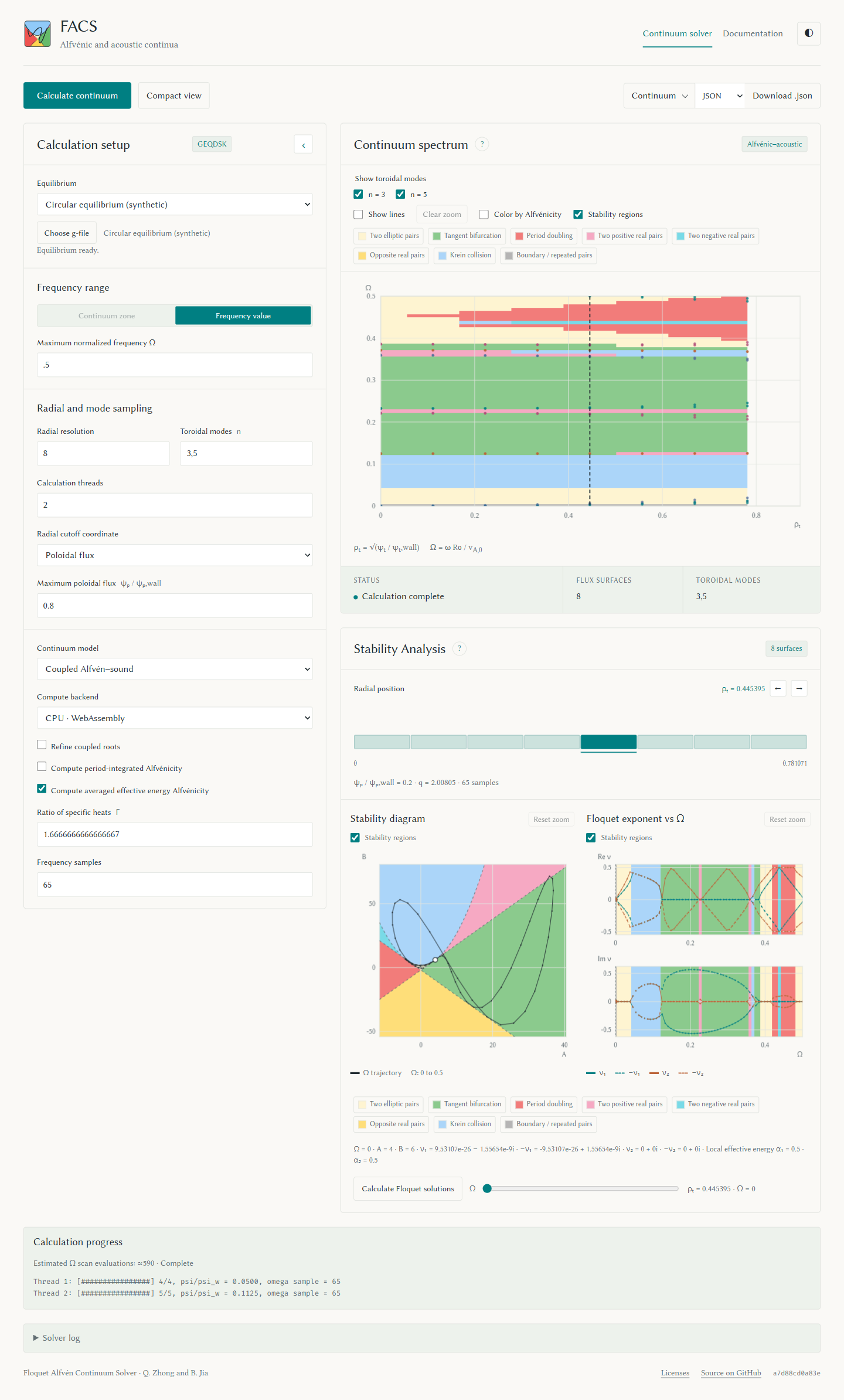
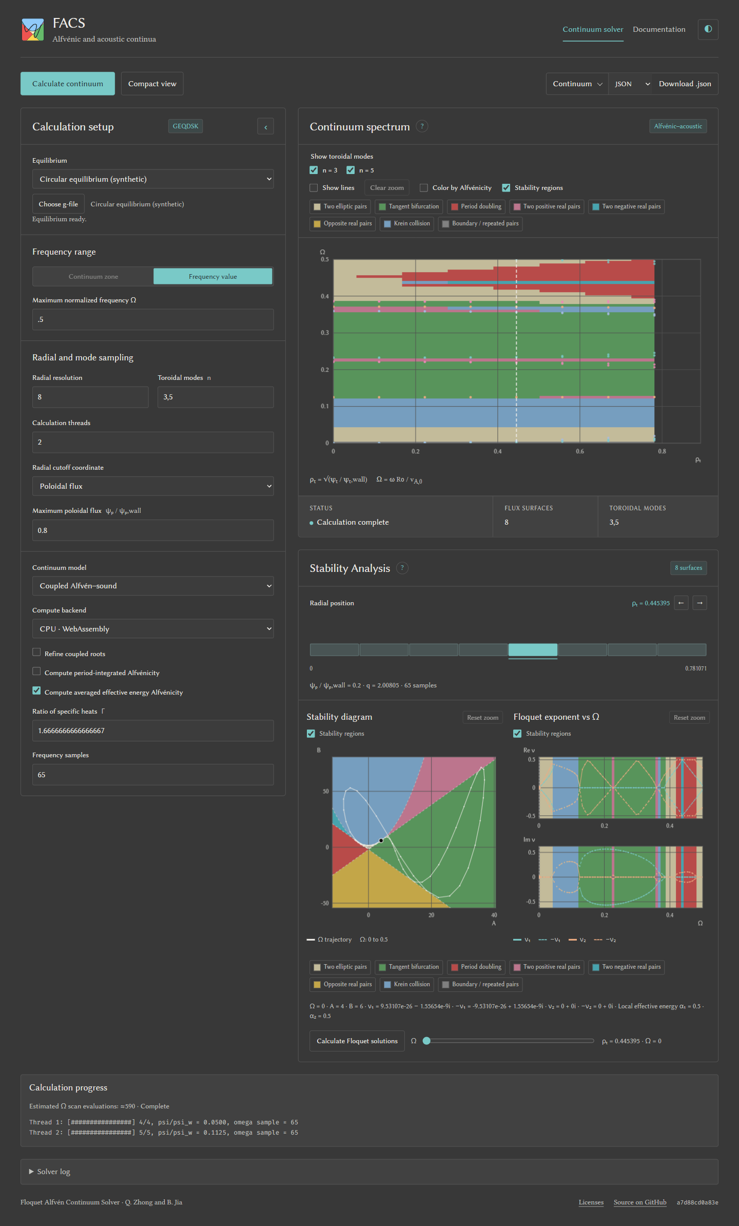
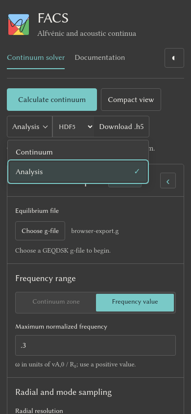
Choose a built-in equilibrium or upload a GEQDSK g-file, set the options, then select Calculate continuum. The plot updates during the run. To download a result, choose Continuum or Analysis, select a format, then choose Download. Continuum offers JSON, NetCDF, and HDF5; Analysis offers text, NetCDF, and HDF5. Binary Analysis includes the continuum and all sampled scans in one file. Downloads keep the completed run's settings, regardless of later form edits or plot filters. Open Solver log to read the calculation messages. See the desktop download control and mobile menu. Hover over a setting or plot heading for help. Tab between settings to show keyboard hints; Escape dismisses them. The ? buttons open setup and plot help; Escape or a click outside closes them. The palette button offers Celadon, Cloisonné, Sorghum, Gromwell, and Carbon. The adjacent light/dark button changes the mode without changing the palette. Both choices are saved across the solver, figures window, license page, and documentation in this browser. Shaded plots use the chosen palette's light colors so their curves remain readable in either mode. The log reports actual frequency scan evaluations, including adaptive probes, separately from retained curve points.
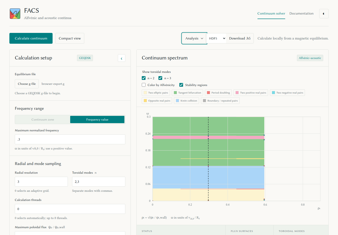
Selecting an uploaded or built-in g-file starts equilibrium spline construction in a worker as soon as the runtime and worker pool are free. The setup panel shows Preparing equilibrium…, then Equilibrium ready. Calculate waits for that same build if needed. Later runs reuse it when settings or the compute backend change. Selecting another file prepares a new equilibrium; completed results keep their original equilibrium and filename for exports and Floquet analysis. Invalid files report an error before a calculation starts.
For the built-in file catalog, see bundled equilibria.
The Compute backend control offers WebAssembly, WebGPU, and paired
f32 WebGPU. See WebGPU precision and fallback before
comparing results.
Foldable screens
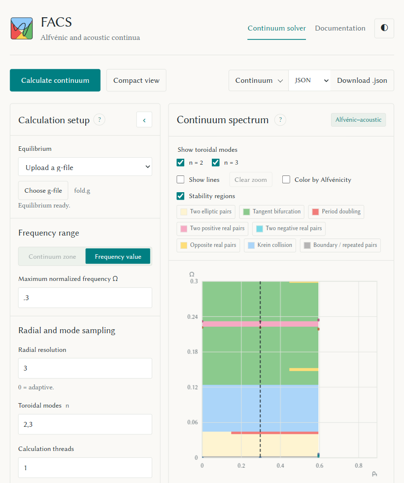
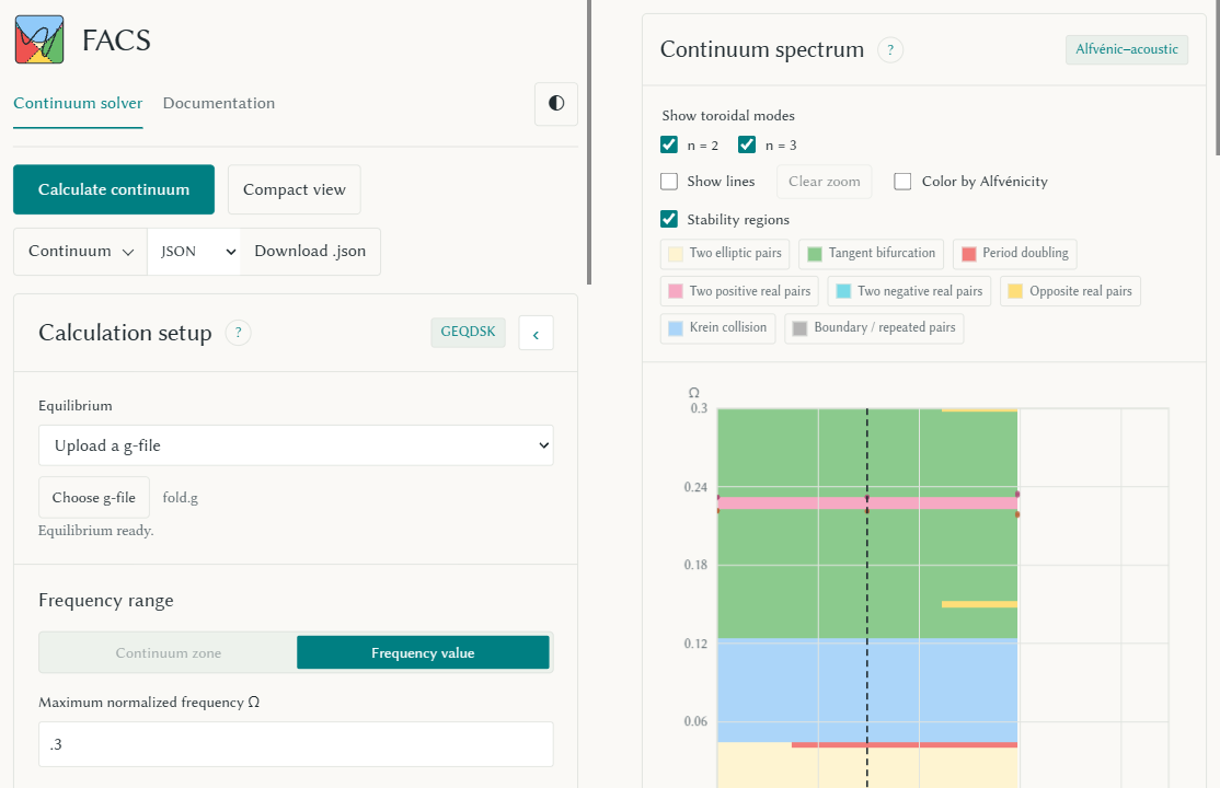
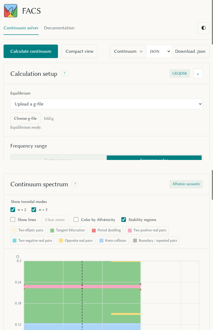
At widths of 660 px and above, setup and plots sit beside each other. Narrower screens use one column. Each panel adapts its controls to its own width.
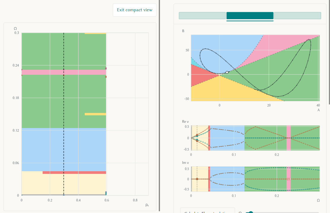
When the browser reports two screen segments through the Viewport Segments API, the app puts controls in the first segment and plots in the second. Each side scrolls on its own, keeping the hinge clear. Rotating to stacked screens puts controls above plots. Compact view puts the spectrum in the first segment and diagnostics in the second; leaving it restores both scroll positions. Folding and rotating keep the calculation, selection, and GPU resources. Browsers that do not report segments use the ordinary responsive layout.
See the unfolded layout, two-display layout, compact plots, and stacked screens. These captures use Chrome's device emulation.
Multiple monitors
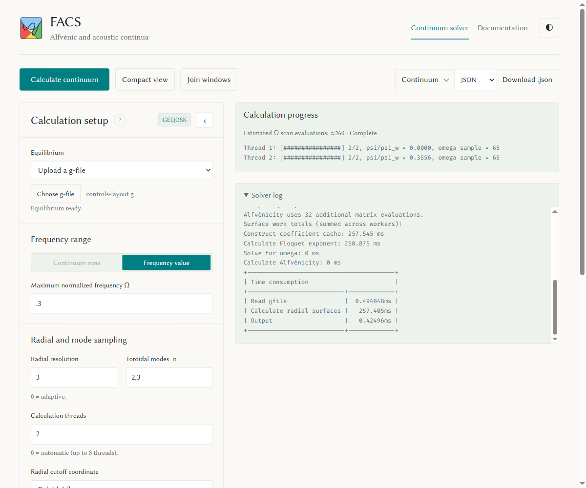
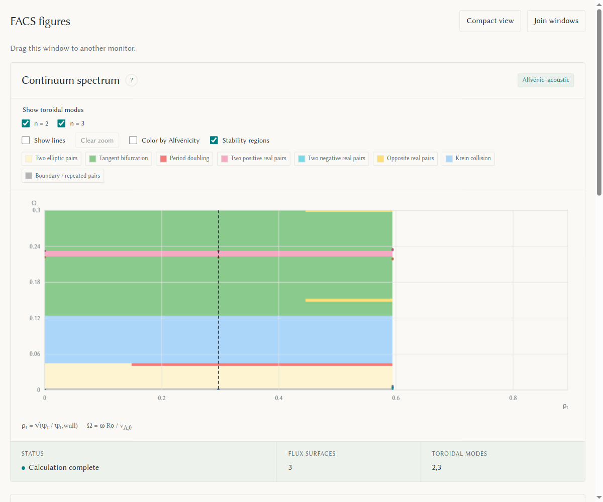
Choose Separate windows to keep setup, calculation controls, downloads, and the log in the original window, and open the plots in a second window. Browsers with the Window Management API can place it on another monitor after you allow screen access. Otherwise, drag the figures window there. If the browser blocks it, allow pop-ups for this site and try again.
In a wide controls window, calculation progress and the solver log sit to the right of setup. Narrow windows stack them below setup.
In browsers that support screen access, an explanation offers Enable screen access or Place manually when permission is not granted. Choose Allow in the browser prompt. If access was blocked, the dialog explains how to allow Window management in the site's browser settings. Escape keeps manual placement. Dismissing the dialog cancels pending placement, even if permission arrives later.
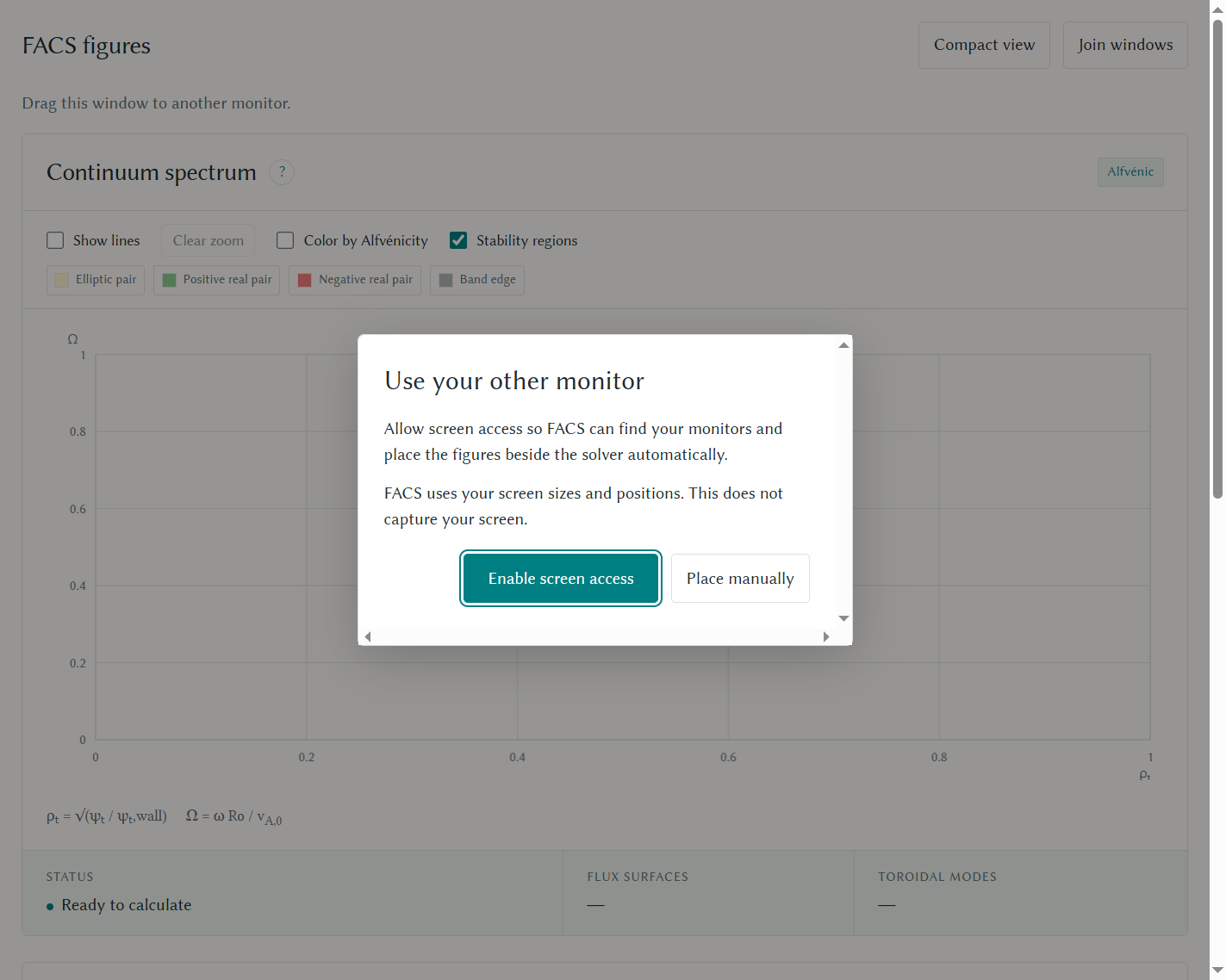
Both windows share one solver and its GPU resources. Splitting keeps the run, selection, and zoom; each window adapts to its display's scale. Compact view affects the figures window while setup stays visible. Join windows in either window, or closing or reloading the figures window, returns the plots to the solver. Closing or reloading the solver closes its figures window.
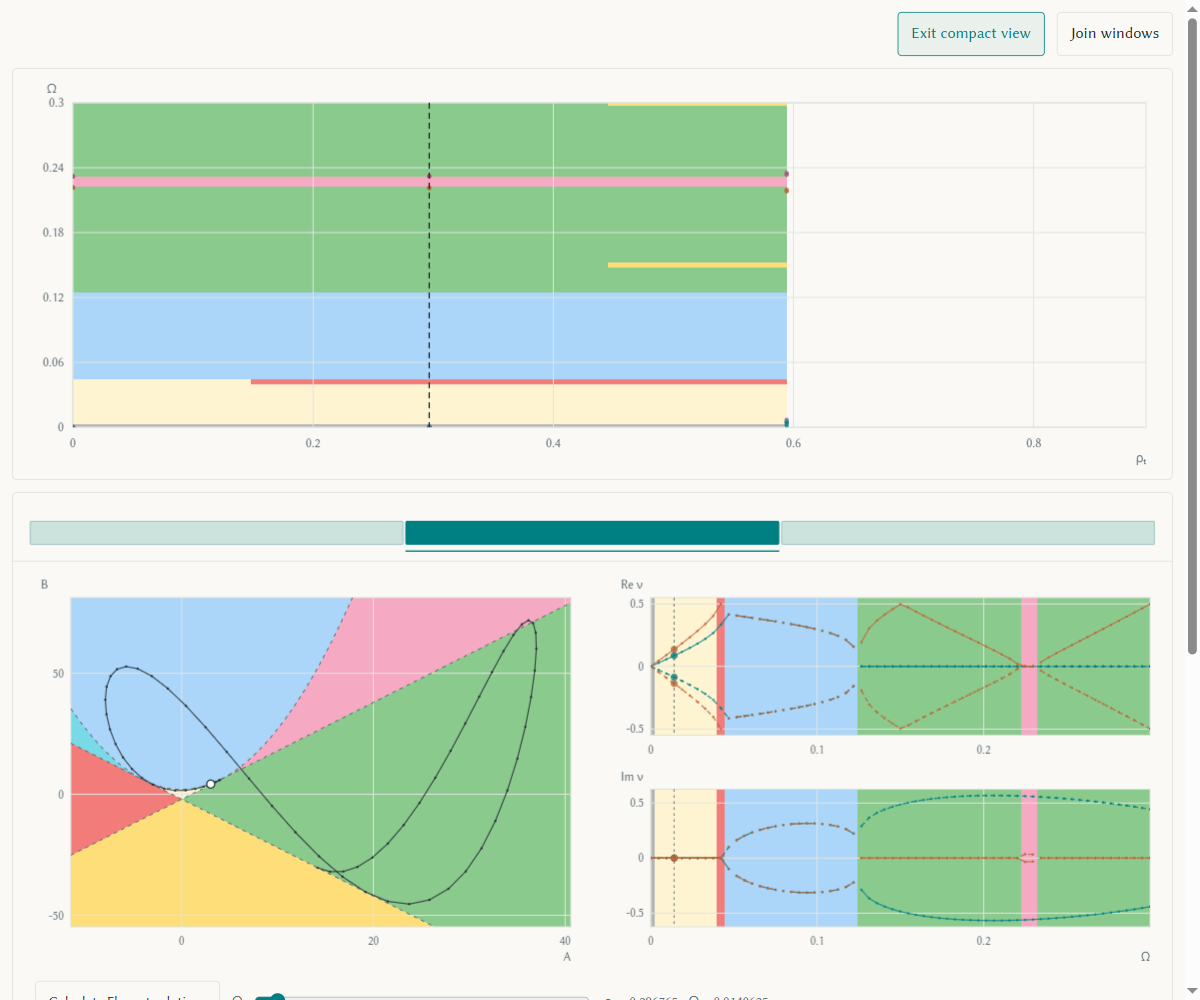
See the controls window, figures window, and compact figures.
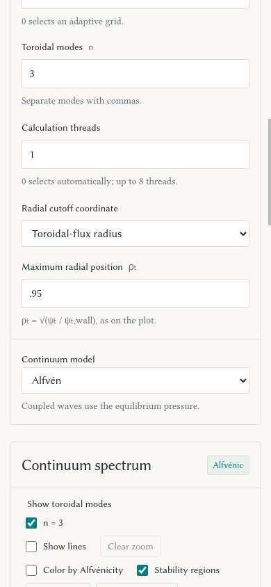
Radial cutoff
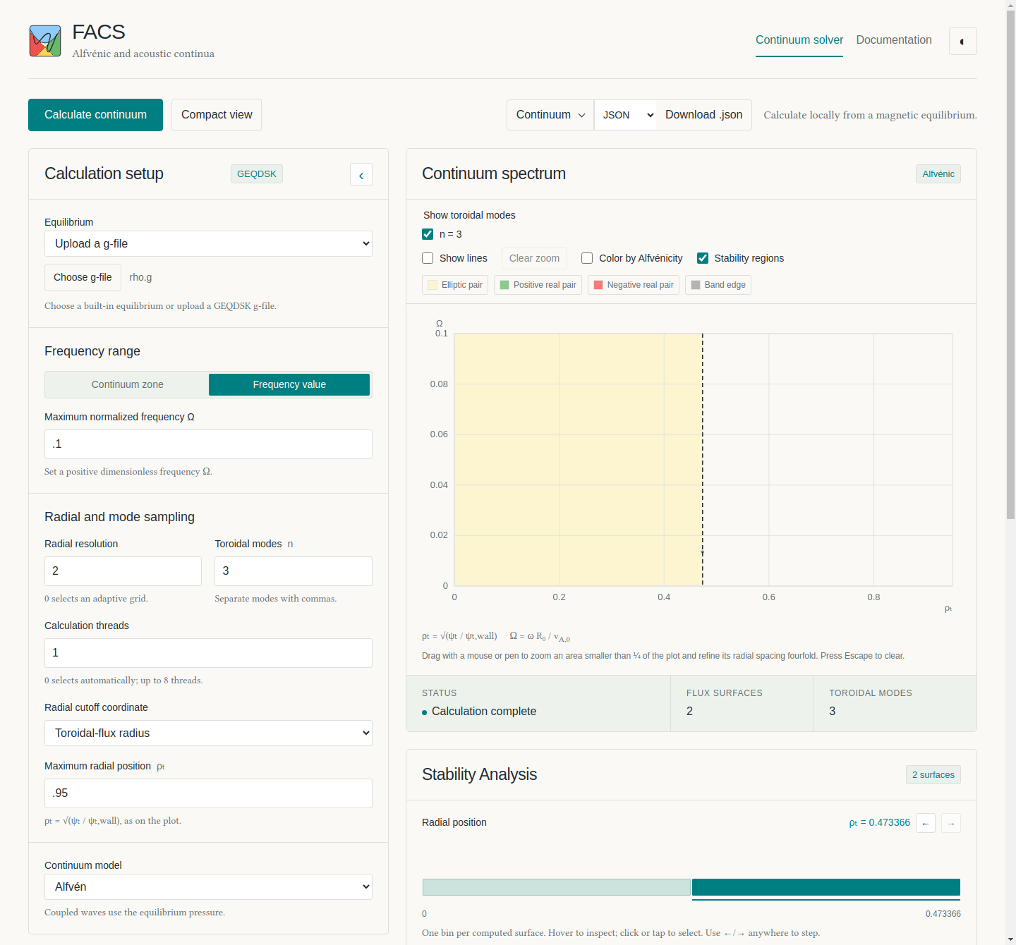
The cutoff defaults to normalized poloidal flux 0.8. To use the plotted toroidal-flux radius instead, choose Toroidal-flux radius under Radial cutoff coordinate, then set Maximum radial position. Zoom refinement uses the same cutoff. Prescribed radial grids approach it without adding a sample exactly at the limit. See the desktop controls and mobile controls.
Spectrum and Alfvénicity
Coupled browser calculations use adaptive frequency sampling by default.
Frequency samples is 0 for adaptive sampling; enter an integer of at
least 2 for that many uniform samples.
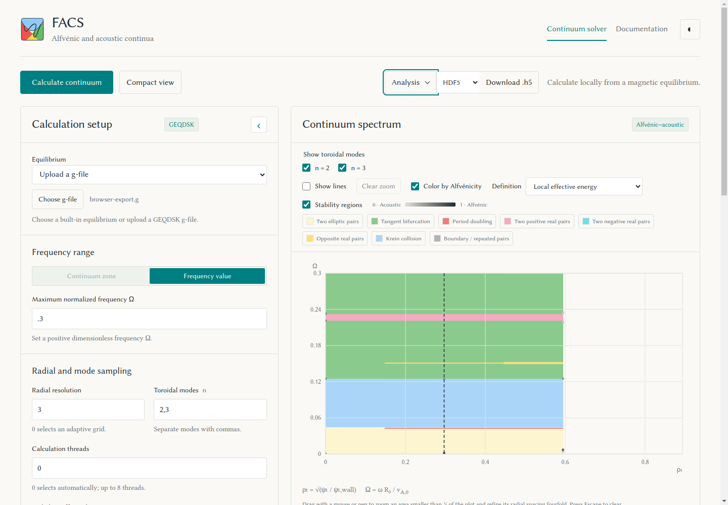
The spectrum shows points by default, with colors cycling by frequency rank
within each toroidal mode. Select Show lines to connect consecutive
points with the same rank. Select Color by Alfvénicity to show acoustic
modes at 0 and Alfvénic modes at 1.
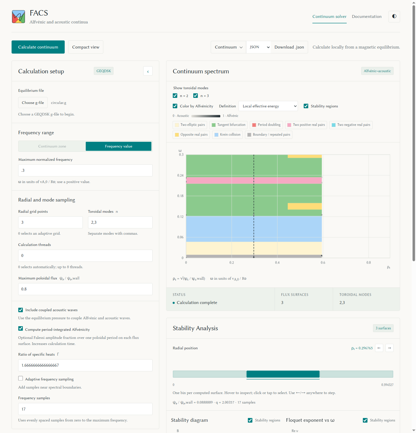
Local effective energy (CSSC) is the default
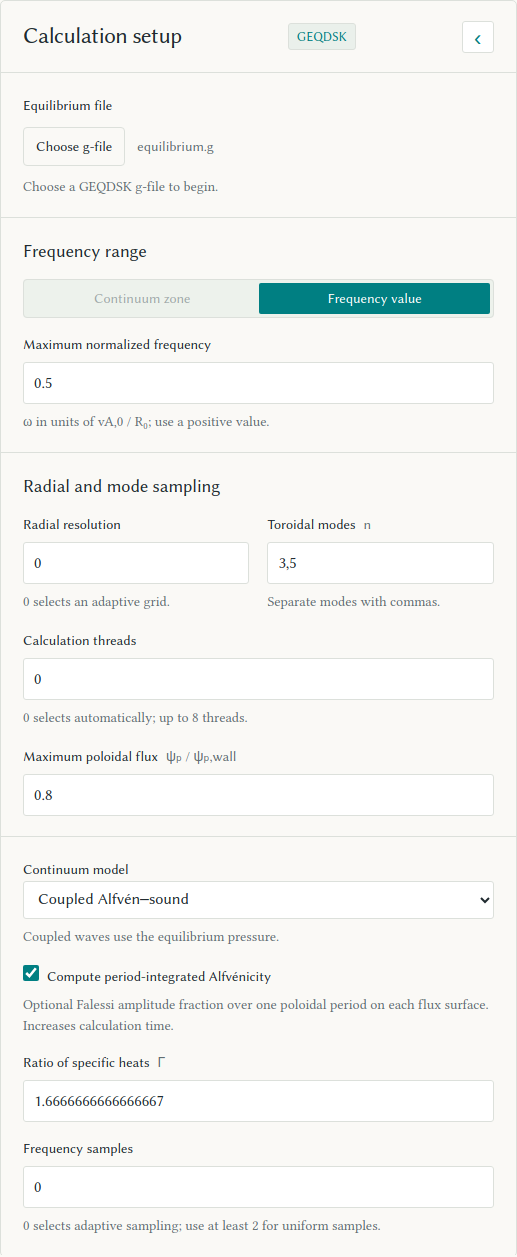
(screenshot). To compute
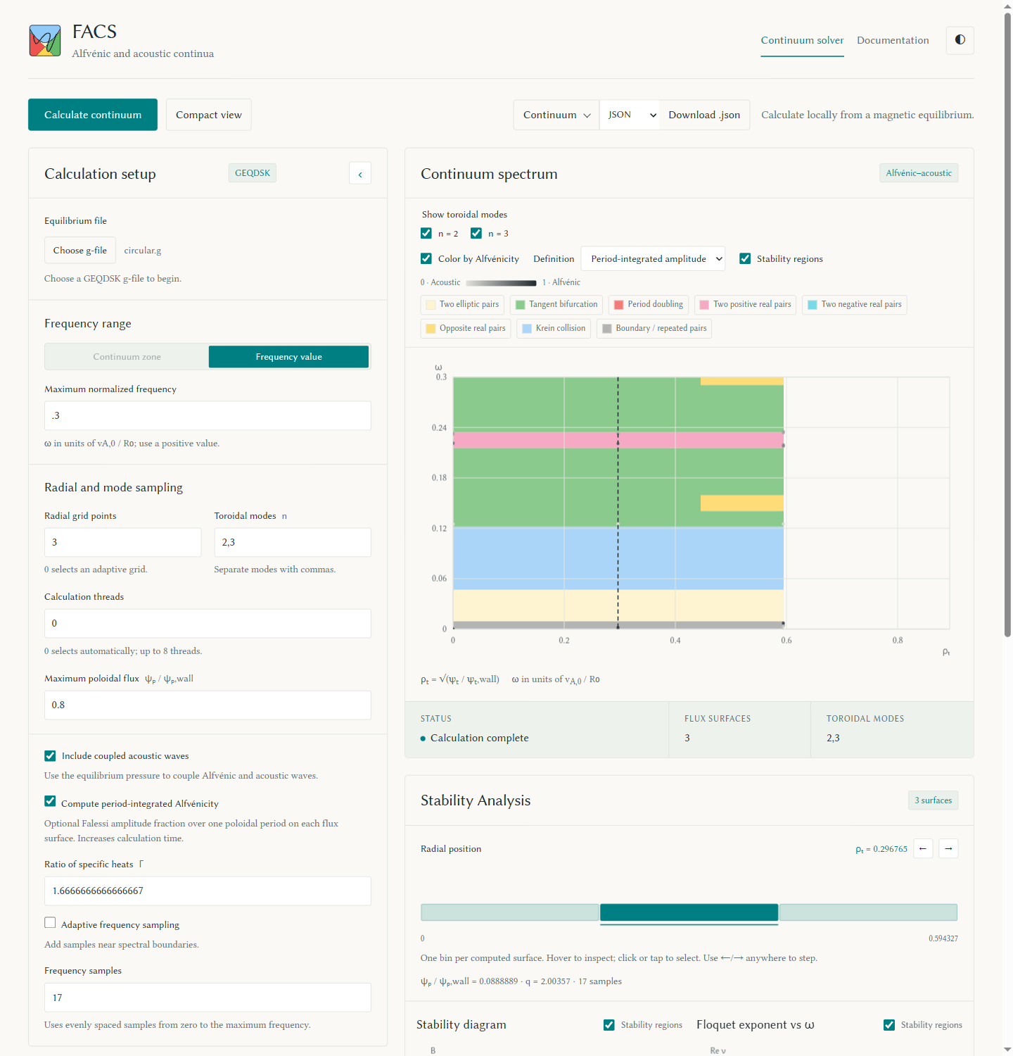
Period-integrated amplitude, select
Compute period-integrated Alfvénicity before starting the calculation.
To compute the third definition, Period-averaged effective energy, select
Compute averaged effective energy Alfvénicity. Then choose a saved measure in
Definition. The amplitude integral uses the
continuum-flux-coordinate amplitude fraction, evaluated by weighting the
existing Boozer θ grid. Switching definitions redraws saved values without
rerunning the solver. The diagnostic readout uses the same selection.
Analysis keeps fields for all three definitions. Each optional period
measure contains nan unless enabled. Both period measures cover one
poloidal period on a single flux surface; local energy uses the starting angle.
See the definitions and
output and plotting for formulas, saved fields, and Python options.
Acoustic modes blend into the background; Alfvénic modes stand out in both modes.
Crosses mark unresolved Alfvénicity. Their legend entry appears only when the
count is nonzero and explains them on hover. The switch redraws existing results.
The horizontal axis ends at the toroidal-flux radius of the chosen cutoff.
Tick marks use simple intervals within that range.
Layout
The browser plot shows finished surfaces from all threads as they arrive.
Use its toroidal-mode checkboxes to show or hide each n. Downloads retain
all calculated modes. Collapse Calculation setup with the arrow in its
heading to make the figures wider and taller; expand it to edit the saved settings.
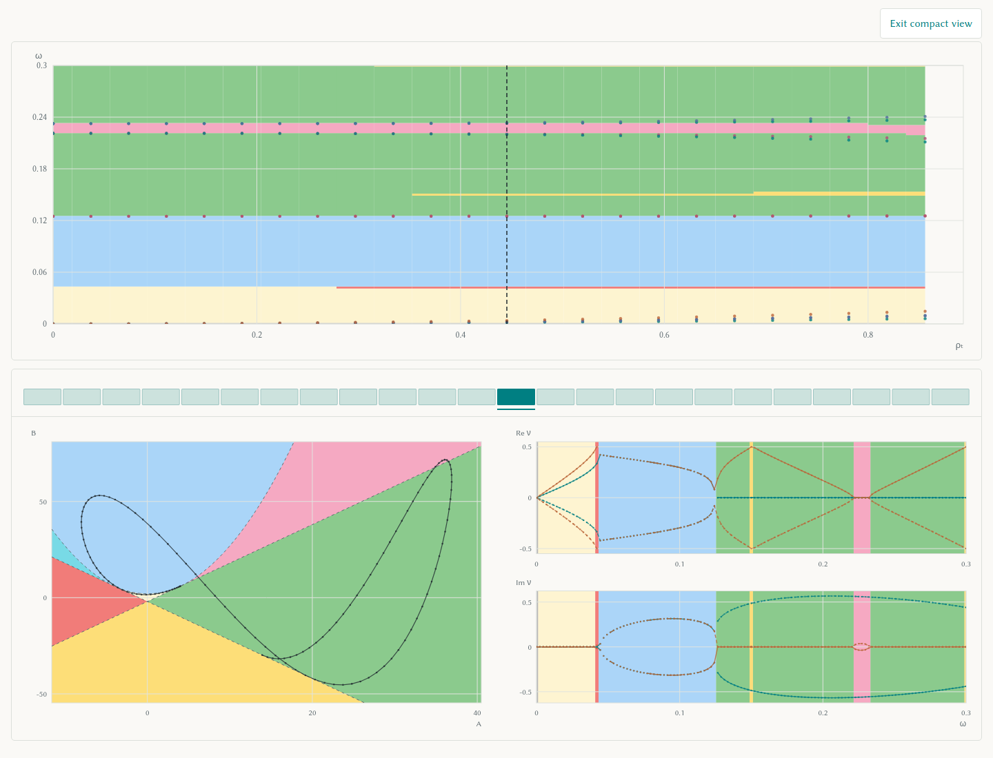
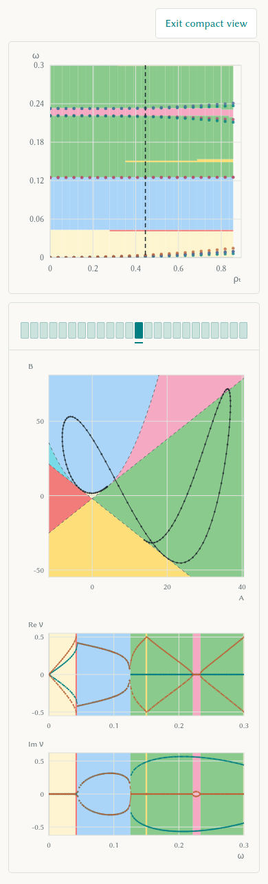
Select Compact view to show only the continuum spectrum, radial control,
matrix stability plot, and Floquet exponent plot. This view hides captions,
legends, setup, and page controls while keeping the plot axes. Select
Exit compact view or press Escape to restore the full page and its settings.
The compact radial control shows only the bins; click or tap a bin, or use
Left/Right, to select a surface.
Stability analysis
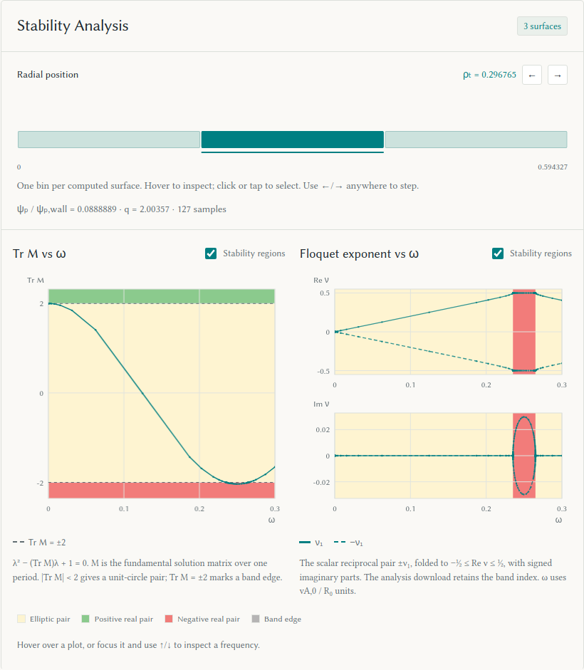
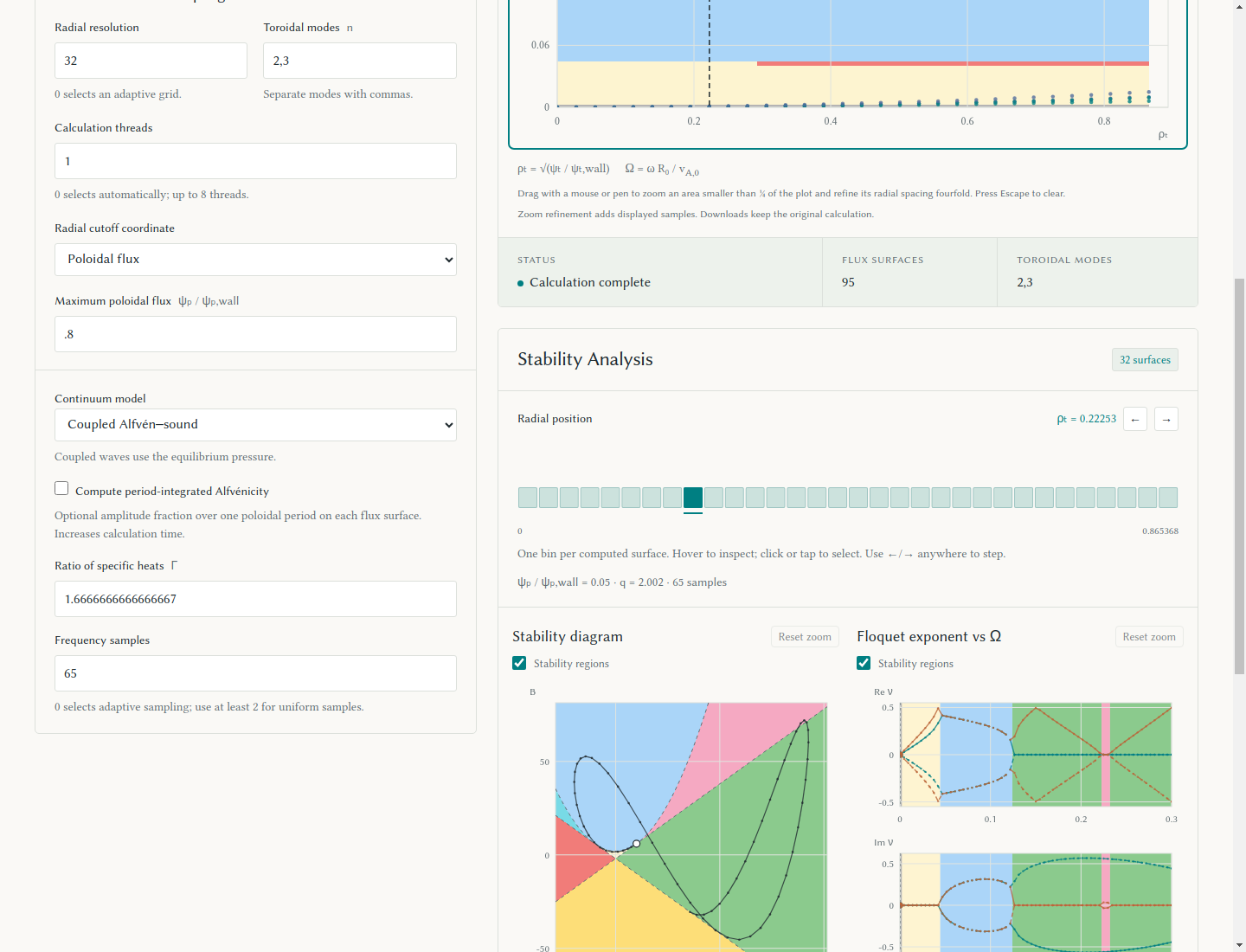
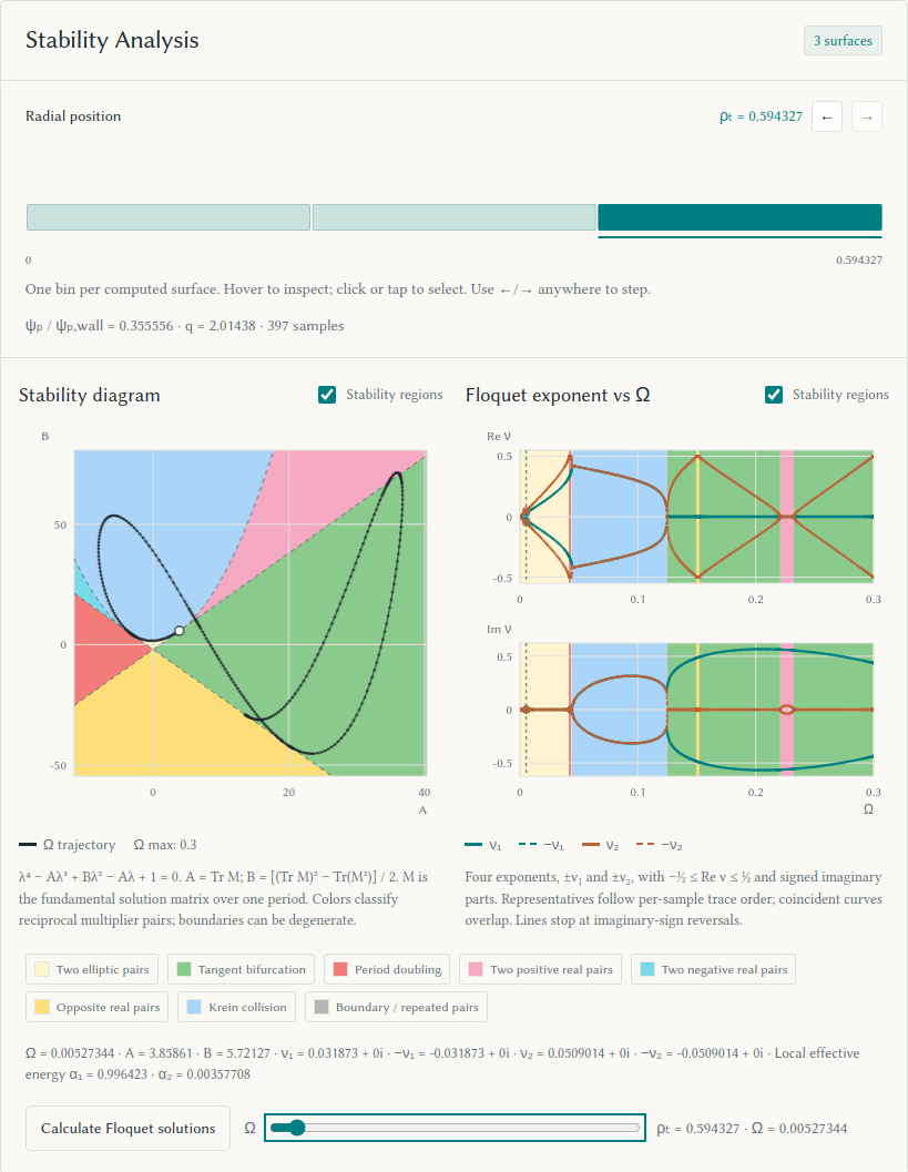
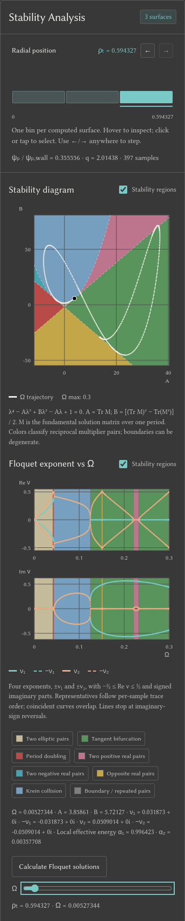
Below the spectrum, Stability Analysis shows the matrix trace (Alfvénic only) or stability diagram (coupled), alongside Floquet exponents versus omega. Each rectangle in the radial selector represents one sampled radius. Hover enlarges a bin and shows its ρₜ value; click or tap selects it. Left/Right and the adjacent buttons step through the radii. The middle available bin is selected by default as surfaces finish. Once you select a bin, the selection stays fixed while that position remains available.
Changing the selection reuses the saved scan. The frequency axis uses the same global
v_A,0/R_0 units as the continuum plot. Hover over either diagnostic plot, or
focus it and use Up/Down, to inspect a sampled frequency in both views.
Left/Right changes the radial position across the page; input fields keep
their normal arrow-key behavior. A vertical dashed line on the continuum
spectrum marks the selected radius.
The exponent plot separates real and signed imaginary parts on symmetric axes.
Both plots fold real parts into [-1/2, 1/2]. Scalar runs show the reciprocal
pair ±nu_1; the analysis download retains its full band index. Coupled runs
show all four exponents ±nu_1, ±nu_2. Coincident curves overlap. Coupled
representatives follow per-sample reciprocal-trace order; these labels do not
track physical Alfvénic or acoustic branches. Lines stop at nonzero imaginary-sign
reversals to avoid joining different representatives through a false zero
crossing. The Broucke diagram applies to the coupled
4×4 matrix and labels its coefficients A = tr(M) and
B = beta = ((tr M)^2 - tr(M^2))/2. Both captions state the characteristic
equation and define M as the fundamental solution matrix over one period.
The coupled equation is lambda^4 - A lambda^3 + B lambda^2 - A lambda + 1 = 0.
The diagram's shaded elliptic interior has two unit-circle pairs; boundary
points can be degenerate. See
the coefficient convention and stability boundaries.
Continuum zoom
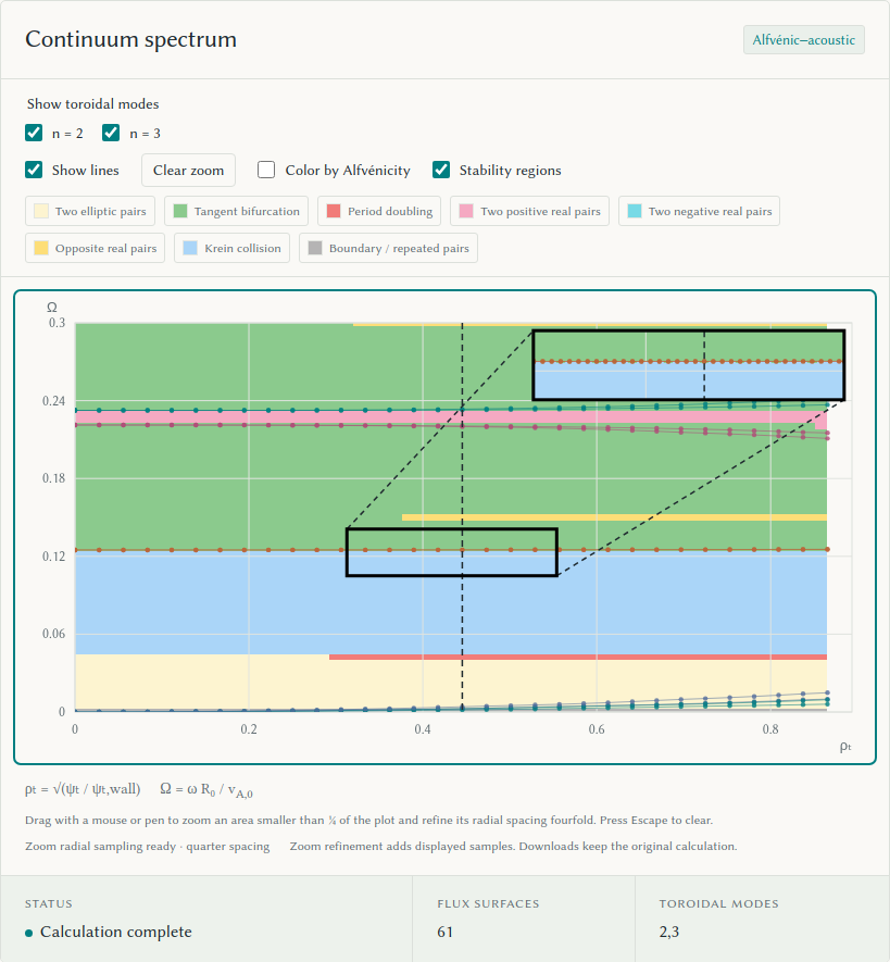
Drag a rectangle with a mouse or pen to show a zoom inset when the selected area is less than a quarter of the plot. The inset sits in the opposite corner, keeps the selection's aspect ratio, and uses at most 40% of the plot width and 80% of its height. Frames and two dashed lines link the views. The inset follows the plot's colors, line visibility, and stability regions. Extra samples appear only in the inset; the main continuum keeps its original points, lines, and shading. Selecting it computes extra radial surfaces in the background, using quarter spacing between the original samples in ρₜ. The solver reuses the loaded equilibrium and the completed run's settings. Repeated or overlapping zooms reuse computed surfaces and scanned frequency intervals; they keep the same original spacing reference. Refinement scans only the selected Ω interval and uses the completed run's calculation thread setting. Narrower windows reduce the scan work while retaining the original frequency resolution.
The radial position selector shows only the zoom interval, including the new surfaces. The stability diagram, Floquet exponent plots, and frequency slider show only samples in the selected Ω interval. These positions also support Floquet solutions. Selection bounds add samples for narrow intervals; the outer flux cutoff remains open, as in the original solve. With rank coloring, coupled refined points use nearby original frequency ranks when the match is clear. Ambiguous points stay grey and do not form lines. Scalar colors follow the absolute continuum zone.
Drag again to replace the zoom; choose Clear zoom or press Escape while the plot has focus to clear it and restore the original radial positions and the full Ω range in stability analysis. If you selected a refined position, the selector moves to the nearest original position. Extra positions stay cached for later zooms and appear in the bins only while a zoom is active. Touch gestures scroll the page. Resizing keeps the selected data range; a new calculation clears it. Zoom refinement affects displayed samples; downloads retain the original calculation. See the zoom inset and radial bins after clearing.
Diagnostic zoom
Drag a rectangle on a stability or Floquet exponent figure to zoom directly to that area. Further drags zoom within the current view. The exponent panes share their Ω limits and keep separate vertical limits. Completed Floquet solution figures also support this zoom. Reset zoom or Escape restores each figure. These zooms use saved data and request no new integrations; their data limits survive resizing. See the diagnostic zoom.
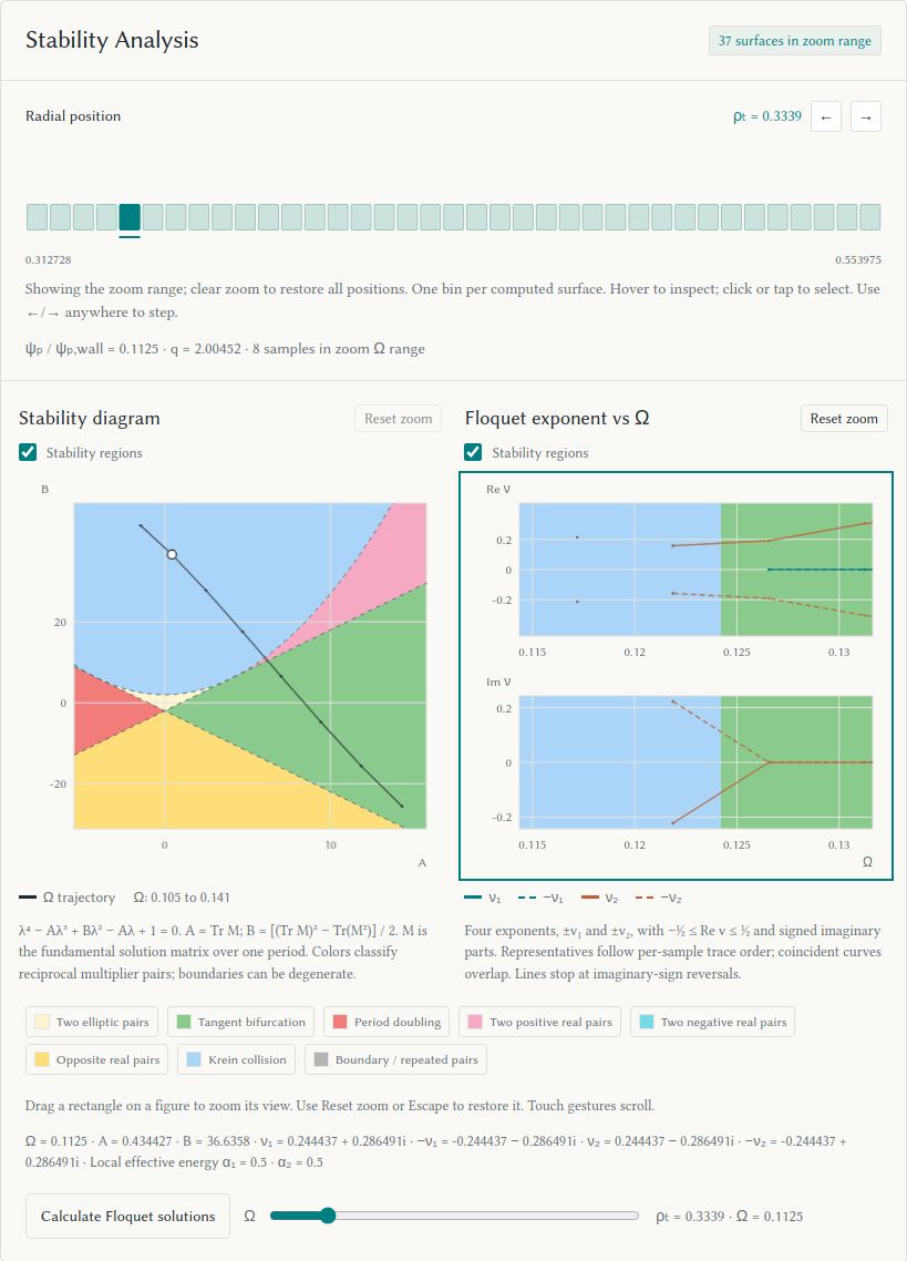
Stability regions
The continuum, stability diagram, and exponent figure each have a
Stability regions checkbox. Select a region in its legend
to hide or show that color. The stability diagram and Floquet exponent plots
share these controls; the spectrum has its own. The palette uses colors from
deck-diagram.png: cream for elliptic pairs, green for an elliptic pair with a
positive real pair, red for an elliptic pair with a negative real pair,
pink and cyan for two real pairs of the same sign, yellow for real pairs of
opposite sign, and blue for a complex quartet. Grey marks boundaries or
repeated reciprocal traces. Region fills and legend swatches share 75% opacity
in light mode and 70% in dark mode.
Alfvénic-only figures use cream, green, and red for an elliptic, positive real,
or negative real pair. The trace plot shows the exact regions at Tr M = ±2.
The stability diagram and scalar trace plot mark the selected Ω with a white
dot in light mode and a black dot in dark mode.
The spectrum and exponent plots use the saved frequency samples, with bin
edges halfway between adjacent samples; the spectrum stops at the outermost
computed radius. Coloring adds no matrix integrations and leaves Alfvénicity
coloring available for the spectrum points.
The figures use dimensionless frequency \(\Omega=\omega R_0/v_{A,0}\), where \(\omega\) is the physical angular frequency. This definition appears below the continuum.
Floquet solutions
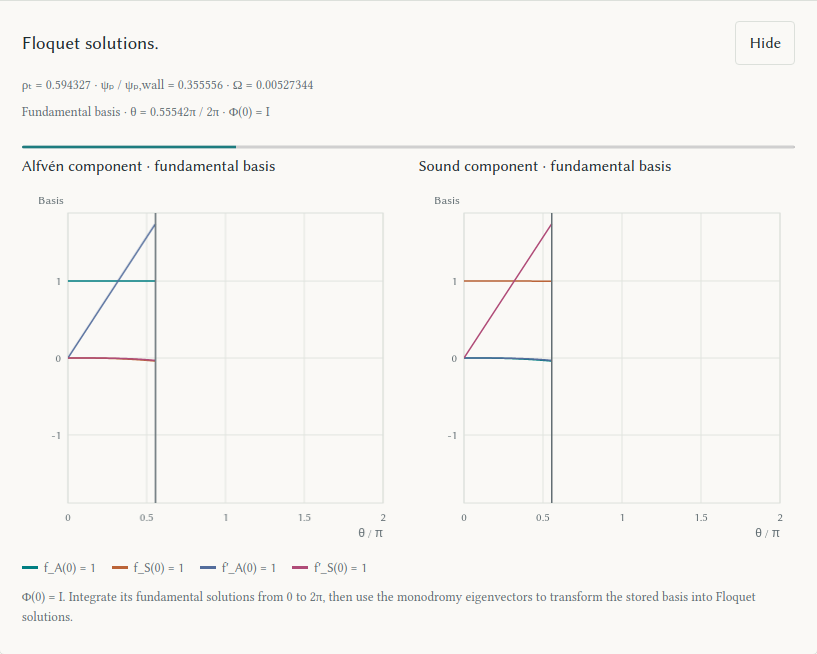
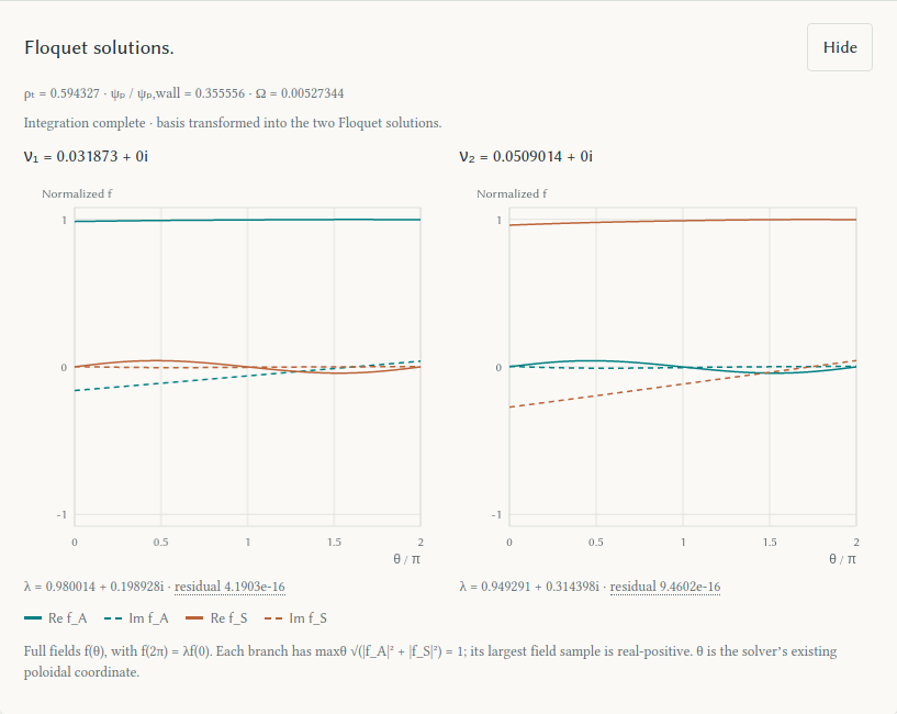
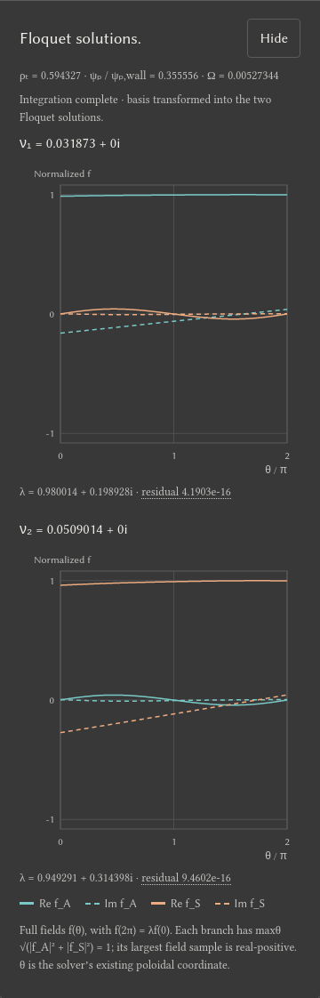
To inspect Floquet solutions, choose a saved radial surface, then select Ω with the slider beside Calculate Floquet solutions. The slider steps through saved samples, which may have uneven frequency spacing. Hover or tap either diagnostic plot, or use ↑/↓ while it has focus, to select the same samples. Both plots keep their markers when the pointer leaves. Choose Calculate Floquet solutions to show the identity fundamental basis advancing from θ = 0 to 2π. After the integration, the monodromy eigenvectors transform the stored basis into two Floquet solutions: ν₁ and ν₂ for coupled waves, or the reciprocal pair ±ν₁ for scalar waves. The raw coupled basis panes show the Alfvén and sound components of all four initial-state columns.
The final plots show real and imaginary parts of the full f_A(θ) and
f_S(θ), with f(2π) = λ f(0). Each branch shares one normalization,
maxθ sqrt(|f_A|² + |f_S|²) = 1; its largest field sample is real-positive.
These are the solver's fields in its existing θ coordinate. Repeated
multipliers can have valid, nonunique Floquet solutions. A profile that fails
eigenvector, closure, or cancellation checks is marked unresolved.
Hover over residual for the relative one-period Floquet
consistency error of the full state, including fields and derivatives.
Each new frequency needs one fresh matrix integration. The browser retains the completed run's equilibrium and caches the selected surface's coefficients, so it does not rebuild the equilibrium or rerun the continuum. Both branches share that pass. Reopening the latest profile uses saved data. The UI keeps responding while the worker integrates; changing radial selection discards a pending view. Later form edits do not change the run used for reconstruction. Floquet solutions are computed only on request and are not added to the continuum or analysis downloads.
Examples: frequency selection, mobile frequency selection, identity basis, coupled Floquet solutions, and mobile view.
Screenshots
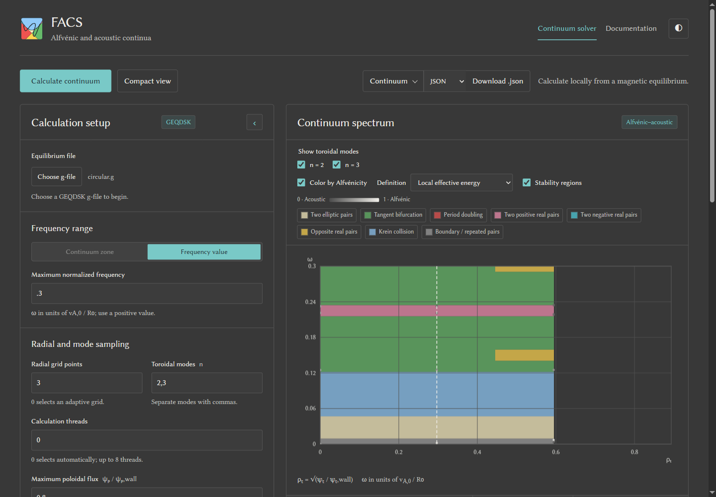
The shared webui appearance: desktop, mobile dark mode, and palette picker.
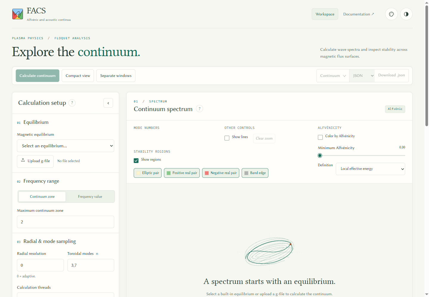
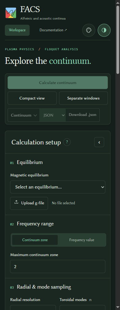
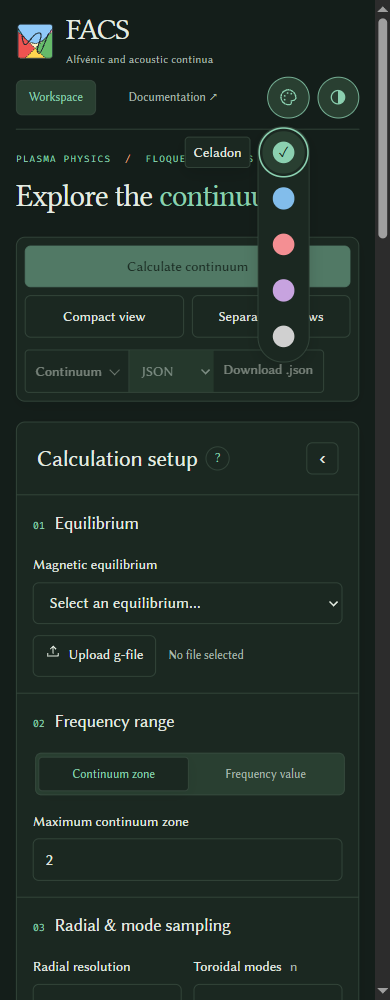
Screenshots: light, dark, mobile, scalar trace, compact, compact mobile, Alfvénicity light, Alfvénicity dark, and period-integrated selection. See also the period-integrated calculation option.