Output formats
FACS writes native continuum text and HDF5/NetCDF results. The browser also offers continuum JSON. Optional Floquet scans can be saved as separate text or embedded in binary files. Plot filters and later form edits do not change the saved calculation.
Native output
Native builds enable binary output when the NetCDF C library with NetCDF-4
support is installed. CMake finds its package configuration or pkg-config
entry. Set -DFACS_ENABLE_NETCDF=OFF to build without it. The numerical
library has no NetCDF dependency; browser exports use bundled Wasm libraries.
The output suffix selects the format: .h5 and .hdf5 select HDF5; .nc
and .nc4 select NetCDF. Both use the same NetCDF-4-compatible HDF5 encoding.
Other suffixes keep the text format. Use --output-format text|hdf5|netcdf
to override the suffix, or auto to infer it.
./build/debug/facs equilibrium.g --model coupled --omega-max 0.5 -n 3 \
    -o continuum.nc --include-floquet
./build/debug/facs equilibrium.g --model coupled --omega-max 0.5 -n 3 \
    --period-integrated-alfvenicity -o continuum.h5 --include-floquet
--include-floquet embeds sampled scans in the binary result. Omit it to
save only the continuum and surface metadata. The separate
--floquet-output option continues to write text. Exporting
binary data does not enable either period measure; each requires its own flag.
Files store all three Alfvénicity measures, surface coordinates and safety factor,
typed solver settings, and optional matrix invariants and signed exponents.
See the binary schema and library writer
for the data layout, normalizations, missing-value rules, and FACS::io API.
Continuum text
The continuum file written by -o starts with the equilibrium poloidal flux
at the wall, then a comment # label_kind continuum_line for coupled runs
or # label_kind continuum_zone for scalar runs. A # line_method comment
records the grouping rule. Each coupled row starts
with n line_index, followed by groups of
rho_t omega alfvenicity, where rho_t = sqrt(psi_t/psi_t_wall) and omega
uses v_{A,0}/R_0. This Alfvénicity is the local effective-energy
measure (CSSC), computed for every coupled point without a separate export flag.
Alfvénic-only rows start with
n continuum_zone, followed by rho_t omega pairs. Readers must select the
point format for the calculation type.
After parallel surface solves, FACS assigns line IDs in radial order. A rank
keeps its ID while it remains present on consecutive surfaces. If it
vanishes, that segment ends; if it returns, it gets a new ID. Thus
line_index identifies a contiguous rank segment and can differ from the
rank after a gap. Text and JSON rows cannot bridge a missing surface.
Rank grouping preserves frequencies and multiplicities and adds no ODE
integrations. It follows frequency order through crossings, so a line can
change polarization. Energy and amplitude Alfvénicities remain
available for coloring and do not affect the connections. These segment IDs
are not poloidal mode numbers or Floquet bands. Saved output records
line_method="frequency_rank" (JSON uses line-method); see
the grouping algorithm and
the binary schema.
Continuum JSON
The browser JSON download also keeps the effective-energy measure,
regardless of the display selection. Coupled records contain line-index;
scalar records contain continuum-zone. Coupled points contain
[rho_t, omega, alfvenicity]; Alfvénic-only points contain [rho_t, omega].
Unresolved character is nan in the text file and null in JSON.
Floquet text
Use --floquet-output PATH to export each sampled frequency and
its Floquet analysis. A directory path selects the filename
floquet-analysis-<g-file name>.
The first line is sound_continuum 0 for Alfvénic only or sound_continuum 1
for coupled waves. Each following line stores one radial position in radial
order, starting with entry_count rho_t, then the entries below. Every complex
value uses two fields, Re Im. Numbers use enough digits to round-trip a double;
this does not increase the calculation's precision.
| Calculation | Fields in each entry | Numeric fields |
|---|---|---|
| Alfvénic only | omega TrM nu_1 nu_2 |
6 |
| Coupled | omega A B mu_1 mu_2 nu_1 nu_2 nu_3 nu_4 alpha_cssc_a alpha_cssc_b alpha_falessi_a alpha_falessi_b alpha_average_a alpha_average_b |
21 |
Here A = TrM, B is the second characteristic coefficient, and
mu = lambda + 1/lambda is a reciprocal trace. Frequencies use v_A,0/R_0
units. Exponents follow reciprocal-pair order: (nu_a, -nu_a) for Alfvénic
only and (nu_a, -nu_a, nu_b, -nu_b) for coupled waves. Scalar exponents keep
their band index; coupled representatives satisfy 0 <= Re(nu) <= 1/2.
The six appended real fields give all three Alfvénicities in reciprocal-pair
order, a then b. A stable pair and its conjugate share each value.
Unresolved values are nan; Falessi values are also nan when disabled or
for unstable pairs. Enable them with --period-integrated-alfvenicity.
Averaged-energy fields require --period-averaged-alfvenicity. Earlier
coupled text files had 19 fields (without the third definition) or 15
(without any Alfvénicity fields); the Python reader accepts both.
Scalar records keep six fields and describe purely Alfvénic waves.
The browser's Analysis → Text download writes this format for all saved
surfaces, regardless of which modes or surface the figures show.
Python plots
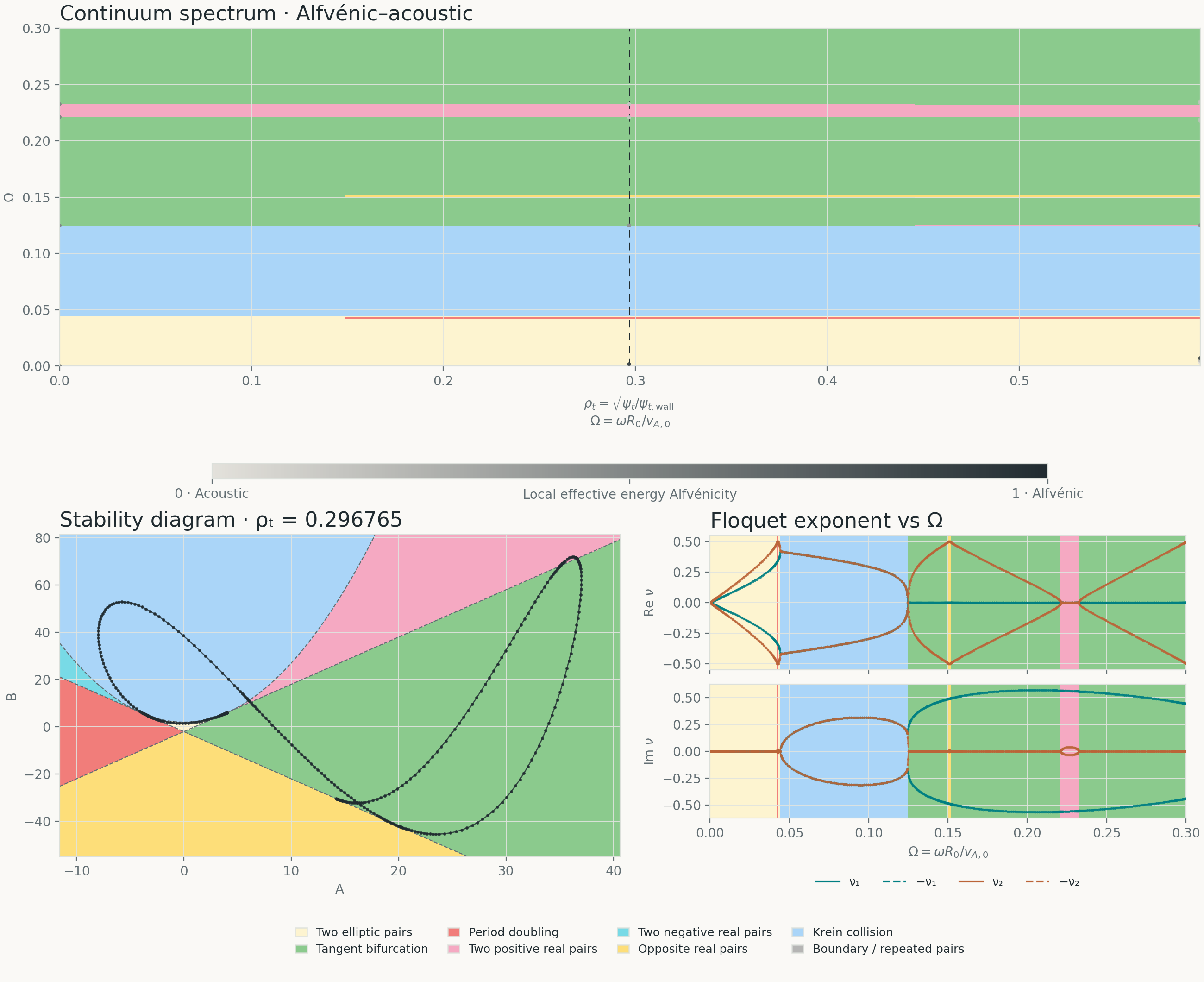
Install the Python dependencies, then plot a native coupled continuum with its sampled Floquet analysis:
python3 -m pip install -r script/requirements.txt
python3 script/plot_facs.py continuum continuum.txt --analysis floquet-analysis.txt \
    --color-by local --rho-t 0.4 -o continuum.png
python3 script/plot_facs.py analysis floquet-analysis.txt --rho-t 0.4 \
    --theme dark -o stability.pdf
Figures use the web app's light/dark colors, stability regions, and signed
Floquet curves. Native text needs --model coupled or --model alfven when
no analysis file supplies the model. Browser JSON records the model in its
line labels.
PNG, PDF, and SVG exports are supported. See Python tools
for filtering, limits, and the reusable reader and plotting APIs.
Example: Python spectrum and diagnostics.
For binary files, install script/requirements-binary.txt. Their model,
settings, and optional embedded scans are read automatically:
python3 -m pip install -r script/requirements-binary.txt
python3 script/plot_facs.py continuum continuum.nc --color-by local -o continuum.png
python3 script/plot_facs.py continuum continuum.h5 --color-by period-integrated -o falessi.pdf
Period-integrated plots use values saved by a run with
--period-integrated-alfvenicity.
Binary schema
FACS schema version 4 stores a calculation in NetCDF-4-compatible HDF5.
The .nc, .nc4, .h5, and .hdf5 extensions use the same encoding.
HDF5 datasets correspond to NetCDF variables; NetCDF supplies dimension
scales. All floating data use IEEE float64, with NaN as _FillValue.
Metadata and settings
The root attributes are format="FACS", schema_version=4,
producer_version, model="alfven" or "alfven_sound", and four int8
flags: falessi_enabled, averaged_enabled, floquet_included, and complete. A reader must
check the schema version and require complete=1. An interrupted export
can leave an incomplete file.
/run/toroidal_mode[mode] is an int32 array. /run holds these typed
attributes after argument defaults have been applied:
| Attribute | Type | Meaning |
|---|---|---|
psi_ratio |
float64 | Resolved poloidal flux cutoff relative to wall flux, including conversion from --rho-max. |
radial_grid_num |
int32 | Requested radial resolution; 0 selects an adaptive grid. |
omega_grid_num |
int32 | Coupled uniform count, or the effective fallback count for adaptive sampling. |
max_omega_value |
float64 | Global dimensionless frequency cutoff. |
max_continuum_zone |
int32 | Scalar zone cap; 0 selects the frequency cutoff. |
adiabatic_index |
float64 | Ratio of specific heats. |
adaptive_omega_grid |
int8 | Adaptive coupled frequency scan flag. |
refine_coupled_roots |
int8 | Full coupled root refinement flag. |
thread_count_requested |
int32 | Requested threads; 0 selects automatically. |
thread_count_used |
int32 | Actual worker count. |
input_file |
text | Input filename supplied by the application. |
compute_backend_requested |
text | Requested calculation backend. |
compute_backend |
text | Accepted backend; mixed means CPU and GPU supplied accepted surfaces. |
scan_precision |
text | float64, float32, paired-f32, or mixed. |
approximate |
int8 | 1 when an approximate GPU backend supplied accepted surfaces. |
frequency_normalization |
text | Omega = omega_physical * R0 / v_A0. |
poloidal_coordinate |
text | boozer_theta. |
cssc_definition |
text | Local signed channel energies at θ=0, compared by absolute value. |
average_definition |
text | Signed channel energies averaged over the full θ period, then compared by absolute value. |
falessi_definition |
text | CFC amplitude fraction evaluated in θ with the squared Jacobian-ratio kernel. |
The saved settings use effective solver values. The CLI default
--omega-samples 0 records adaptive_omega_grid=1 and omega_grid_num=1025
for coupled runs. A positive count records adaptive_omega_grid=0 and that
uniform count. The CLI sentinel zero is never passed to the coupled sampler.
These values and coordinates support analysis and plotting. They do not store the full equilibrium or a density needed to recover physical frequency. See WebGPU metadata for fallback conventions.
Surfaces and continuum
surface indexes calculation surfaces in their original order. Equal radii
remain separate surfaces. line indexes continuum lines sorted by
(n,line_index). Ambiguous connections start new line IDs. point indexes
their concatenated points. All indices and starts are zero-based.
| Path | Shape | Type |
|---|---|---|
/equilibrium/psi_wall |
scalar | float64 |
/surfaces/rho_t |
[surface] |
float64 |
/surfaces/psi_over_psi_wall |
[surface] |
float64 |
/surfaces/q |
[surface] |
float64 |
/continuum/n, /continuum/line_index |
[line] |
int32 |
/continuum/point_start, /continuum/point_count |
[line] |
int64 |
/continuum/surface_index |
[point] |
int64 |
/continuum/omega |
[point] |
float64 |
/continuum/alfvenicity_cssc |
[point] |
float64 |
/continuum/alfvenicity_falessi |
[point] |
float64 |
/continuum/alfvenicity_average |
[point] |
float64 |
psi_wall is the outward normalized poloidal wall flux,
psi_p_wall/(R0^2 abs(B0)). The plotted radius is
rho_t=sqrt(psi_t/psi_t_wall). psi_over_psi_wall uses poloidal flux;
q retains its sign. omega is the global dimensionless frequency Ω,
normalized to v_A0/R0. Each numeric variable has units and long_name
attributes explaining its convention.
For line i, slice point arrays from point_start[i] to
point_start[i]+point_count[i]. Recover radii with
surfaces/rho_t[continuum/surface_index]. /continuum has index_base=0
and label_kind="continuum_zone" for scalar waves or "continuum_line"
for coupled waves. Scalar line_index stores the continuum zone. Coupled
line_index is a nonnegative ID for a contiguous frequency-rank segment,
assigned separately for each n. The lowest root joins the lowest on the
next surface, the second joins the second, and so on. A missing rank ends
its segment; a returning rank gets a new ID. Consequently line_index need
not equal the frequency rank after a gap.
The /continuum/line_method text attribute records "frequency_rank" for
coupled runs and "continuum_zone" for scalar runs. Earlier schema-3 files
may omit it; the reader returns line_method=None. The attribute distinguishes
the grouping rule without changing the schema layout. Text stores it in a
# line_method comment; JSON uses line-method. Frequency-rank lines
can change polarization at a crossing. Alfvénicity controls optional coloring,
not the grouping. See the grouping algorithm.
Version 1 used /continuum/label and label_kind="frequency_rank" for
coupled output. Version 2 used branch_index, band_index, and
label_kind="floquet_branch_band". Python readers accept all four versions:
new curve IDs and old ranks are integers; version-2 coupled labels remain
(b,j) tuples. Legacy unresolved pairs remain separate rows. Floquet scan
arrays keep their per-sample reciprocal-trace order in all four versions.
Optional Floquet analysis
When floquet_included=1, /floquet holds a concatenated scan array and
per-surface starts and counts. Counts can be zero. The sample grid can
differ between surfaces; no padding or interpolation is applied.
Variable under /floquet |
Shape | Type |
|---|---|---|
sample_start, sample_count |
[surface] |
int64 |
sign |
[sign=2], values +1,-1 |
int32 |
omega, A, B |
[sample] |
float64 |
nu_real, nu_imag |
[sample,pair,sign] |
float64 |
mu_real, mu_imag |
[sample,pair] |
float64 |
alfvenicity_cssc, alfvenicity_falessi, alfvenicity_average |
[sample,pair] |
float64 |
There is one reciprocal pair for scalar waves and two for coupled waves.
The stored ν values follow the solver: scalar exponents retain band indices;
coupled representatives are folded. The last dimension stores explicit
+nu,-nu partners, including signed imaginary parts and signed zero.
Pair order follows each sample's reciprocal traces, without physical branch
tracking or further phase folding.
A=tr(M), B=((tr M)^2-tr(M^2))/2, and mu=lambda+1/lambda for the
one-period fundamental matrix M. Scalar conventions are B=NaN,
mu=A+i0, and CSSC Alfvénicity 1 for a pure Alfvénic wave.
Continuum and scan arrays keep three independent measures:
| Field | Definition | Availability |
|---|---|---|
alfvenicity_cssc |
Local effective energy at θ=0 (default) | Always computed; scalar convention is 1. |
alfvenicity_falessi |
Period-integrated amplitude | Requires --period-integrated-alfvenicity. |
alfvenicity_average |
Period-averaged effective energy | Requires --period-averaged-alfvenicity. |
The /run definition attributes record each formula and normalization.
Both optional arrays contain NaN when disabled or for scalar runs. When
enabled, NaN means unavailable or unresolved. The two period measures share
one propagation pass when both flags are set. Falessi evaluates the
continuum-flux-coordinate norm on the existing Boozer θ grid over [0,2*pi] with
\(W=(J_\theta/J_\eta)^2\propto|\nabla\psi|^{-4}\).
Earlier files contain an unweighted θ norm under the same field name;
their /run/falessi_definition attribute records that earlier formula.
Schema 4 adds the average arrays and flag and restores local CSSC values.
Readers require those new fields in schema 4. Schemas 1–3 without an average
return NaN for the third definition. Some schema-3 files instead stored
averaged CSSC values, identified by a /run/cssc_definition beginning
|<E_A>|. For coupled files, Python returns those values as
alfvenicity_average and fills the unavailable local values with NaN.
Scalar CSSC remains 1. Earlier text/JSON lacks this metadata, so the reader
preserves its energy column without inferring a definition.
Browser downloads
The browser uses the same writer in a separate Wasm worker. Choose Continuum → NetCDF/HDF5 for continuum and surface data, or Analysis → NetCDF/HDF5 to include every saved scan. JSON continuum and text analysis remain available from the same control.
The export keeps the original calculation surface indices, mode-group order, and empty scans. The plots may merge repeated radii or hide modes; those display choices do not change the file. Settings come from the completed run, with the requested and actual thread counts recorded separately. File export performs no integrations and never enables a period measure.
Library writer
Link FACS::io and include output_file.h. Construct facs::OutputFile
with the path, SolverSettings, toroidal modes, optional source filename,
and whether to include scans. For scans, set capture_scan=true. Call
append_surface from surface_ordered, then call finish(result). For scan
export, do not set surface_ready: that callback takes diagnostic ownership
before surface_ordered. The writer streams each scan and retains only
surface fluxes and continuum surface indices.
Calls into NetCDF are serialized across writers. finish checks writes and
close; destruction closes an unfinished file without marking it complete.
The numerical FACS::lib target has no NetCDF dependency.