Python output tools
Use Python 3.10 or newer. Install the dependencies with:
python3 -m pip install -r script/requirements.txtFor HDF5/NetCDF files, install script/requirements-binary.txt instead. It
adds h5py. The reader can also use netCDF4 when h5py is absent; either
backend reads both extensions.
Plotting
Plot a native continuum with effective-energy coloring:
python3 script/plot_facs.py continuum continuum.txt --model coupled \
    --color-by effective-energy -o continuum.png
Add an analysis file to include stability backgrounds and the trace/Broucke
and Floquet panels, like the browser. The analysis header supplies the model,
so an explicit --model coupled or --model alfven option is optional:
python3 script/plot_facs.py continuum continuum.txt --analysis floquet-analysis.txt \
    --rho-t 0.4 --color-by effective-energy -o continuum.png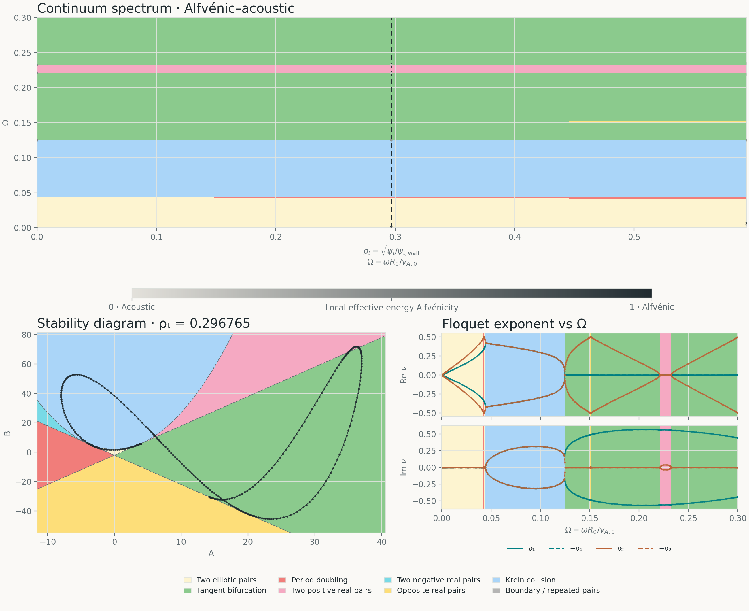
All frequency axes use \(\Omega=\omega R_0/v_{A,0}\), where \(\omega\) is the physical angular frequency. The definition appears below the continuum and on the Floquet frequency axis.
Binary files identify their model and keep all three Alfvénicity definitions. When they contain Floquet scans, the plotting command adds those panels automatically:
python3 script/plot_facs.py continuum continuum.nc --color-by effective-energy -o spectrum.png
python3 script/plot_facs.py continuum continuum.h5 --color-by period-integrated \
    --rho-t 0.4 --theme dark -o spectrum.pdf
python3 script/plot_facs.py analysis continuum.nc --rho-t 0.4 -o stability.svg
Binary plots offer three definitions:
- Local effective energy (default):
--color-by localoreffective-energy. - Period-integrated amplitude:
--color-by period-integrated. - Period-averaged effective energy:
--color-by period-averaged.
The period choices require --period-integrated-alfvenicity and
--period-averaged-alfvenicity, respectively, during the solver run.
The two measures cover the full poloidal period on one flux surface.
Text and JSON lack definition metadata, so their existing energy column
uses the neutral label Effective energy. The reader and plotter use saved values without running
any integrations.
Plot browser JSON, choose toroidal modes, or export one surface's diagnostics:
python3 script/plot_facs.py continuum continuum.json --toroidal-modes 3,5 --theme dark \
    --omega-max 0.5 -o spectrum.svg
python3 script/plot_facs.py analysis floquet-analysis.txt --rho-t 0.4 \
    --theme dark -o stability.pdf
--rho-t selects the nearest saved surface; each figure labels the actual
radius. Without it, diagnostics show the middle nonempty radius. Binary
figures use the saved radial extent and frequency cutoff. For text and JSON,
--rho-max defaults to at least 1 and --omega-max to the largest saved
frequency; those exports do not store the calculation limits. Set limits
explicitly to override them. --no-stability hides region fills.
The solver and plotting command both use --model alfven|coupled and
-n, --toroidal-modes LIST. Mode lists contain comma-separated nonzero signed
32-bit integers; --toroidal-modes -3,5 and --toroidal-modes=-3,5 both work.
Plotting infers the model from saved metadata or an analysis file when
--model is omitted. The earlier model and mode-list option spellings have
been removed.
Points use a stable color per toroidal mode by default. --color-by effective-energy
uses the browser's acoustic-to-Alfvénic gradient and crosses for unresolved
values. Text and JSON continuum exports contain CSSC values; binary exports
also support --color-by period-integrated and --color-by period-averaged.
The reader exposes all three definitions from analysis files. Older coupled analysis files without
Alfvénicity columns remain usable for stability and Floquet plots.
The plotting code uses the web app's palette, scaled stability tolerance, nonuniform sample midpoints, signed exponents, and imaginary-sign line breaks. It folds scalar phases only for display. Stability fills stop at the first and last saved radial/frequency samples. It selects the last scan at repeated radii, as the browser does. Fonts use local fallbacks and need no downloads.
From the repository root, start Python with PYTHONPATH=script python3
and use the same figures:
from facs_output import read_continuum, read_floquet
from plot_facs import plot_continuum, plot_analysis

analysis = read_floquet("floquet-analysis.txt")
data = read_continuum("continuum.txt", coupled=analysis.coupled)
figure = plot_continuum(data, analysis=analysis, rho_t=0.4, color_by="effective-energy")
figure.savefig("continuum.pdf")
figure = plot_analysis(analysis, rho_t=0.4, theme="dark")
figure.savefig("stability.svg")Reading
facs_output.py reads native continuum text, browser continuum JSON, text
Floquet analysis, and binary results. Import it from this directory or add
script/ to your Python path:
from facs_output import read_continuum, read_floquet

analysis = read_floquet("floquet-analysis.txt")
continuum = read_continuum("continuum.txt", coupled=analysis.coupled)
surface = analysis.surface_at(0.4)  # Nearest available rho_t.
print(surface.rho_t, surface.omega, surface.nu)
Native continuum text requires coupled=True or coupled=False; its wall-flux
header alone does not record the model. New text adds a label_kind comment.
JSON infers the model from line-index or continuum-zone. Both readers
preserve row order and repeated axis points. Coupled labels are radial curve
IDs for contiguous frequency-rank segments. Equal ranks join on successive
surfaces; disappearing ranks end their segment. line_index can differ
from the rank after a gap.
The readers also accept schemas 1–3 and earlier text/JSON: version-2
coupled (b,j) labels remain tuples, and old frequency ranks remain integers.
Each continuum line provides n, label, and a points array containing
rho_t, omega and, for coupled runs, CSSC Alfvénicity. JSON null
Alfvénicities become NaN. ContinuumOutput.label_kind records the index
convention; line_method records the grouping rule when saved. Current
coupled files use "frequency_rank"; older files can return None.
New coupled IDs draw connected curves; scalar zones draw segments only when
saved surface indices establish adjacency. Older formats remain scatter.
read_floquet reads the sound_continuum header and counted records. It accepts
current coupled records with 21 numeric fields and older records with 19
or 15. Missing definitions have NaN values. Scalar records keep six fields.
Each surface contains global omega, two coefficients columns (A = Tr M,
B), all signed complex exponents in nu, reciprocal traces in mu, and
two columns each for alfvenicity_cssc, alfvenicity_falessi, and
alfvenicity_average. Scalar B
is NaN. Disabled or unresolved Alfvénicities stay NaN. Scalar exponents retain
band indices; the reader adds no phase folding. Coupled representatives
already follow the solver's folded convention.
unique_surfaces() returns the last record at each radius, as the browser
does. surface_at(rho_t) selects the nearest nonempty scan and reports its
actual radius. Without a radius it selects the middle available surface.
Text analysis files do not contain safety factor or poloidal-flux coordinates.
Binary files use the shared FACS schema. Both reader
functions detect them by file signature, so the extension need not match.
read_continuum(path) infers the model. Its surfaces table has rho_t,
psi_over_psi_wall, and q arrays. Each line adds surface_index,
alfvenicity_falessi, and alfvenicity_average arrays without changing the existing points columns.
Each binary Floquet surface adds its original surface_index,
psi_over_psi_wall, and q. Duplicate surface identities remain distinct;
unique_surfaces() still provides the browser's selection rule.
For schema-3 coupled files whose cssc_definition records a period average,
the reader moves that value to alfvenicity_average and returns NaN local
values. Older files without averages return NaN for the third definition.
Scalar CSSC values remain 1.
Both binary outputs expose metadata["root"] and metadata["run"].
Settings are Python scalar values; toroidal_mode is an integer array.
The reader rejects unsupported schemas, incomplete calculations, and invalid
shapes or ragged indices. Scalar binary scans use the schema conventions
mu=A+i0, CSSC 1, and both optional definitions NaN. Their Alfvénicity arrays retain
two columns, with the unused second pair filled by NaN.
data = read_continuum("continuum.nc")
analysis = read_floquet("continuum.nc")  # Requires --include-floquet at export.
print(data.metadata["run"]["psi_ratio"])
print(data.lines[0].alfvenicity_falessi)
print(analysis.surfaces[0].q)
Pass backend="h5py" or backend="netcdf4" to either reader to select an
installed API. Text/JSON readers need neither package.
Run the reader and plotting tests from the repository root:
python3 -m unittest discover -s test -p '*_test.py'Binary checks need an installed backend and the output-file-test fixture
generator. CTest supplies its path; direct unittest runs look in
build/debug/test/ or use FACS_OUTPUT_FIXTURE.
Native timing comparisons
benchmark_facs.py compares native coupled solves with the same input and
options. It needs only Python's standard library. Build each executable in
Release mode. Replace BEFORE_EXECUTABLE and AFTER_EXECUTABLE
with the executables to compare, and REPORT_FILE with the output filename:
python3 script/benchmark_facs.py equilibrium.g \
    --executable before=BEFORE_EXECUTABLE \
    --executable after=AFTER_EXECUTABLE \
    --omega-max 0.5 --omega-samples 0 --radial-resolution 8 \
    --toroidal-modes 3,5 --threads 1 --analysis \
    --output REPORT_FILE
The script interleaves three runs of each build and saves commands, logs,
integration counts, and median solve times. Solve time covers radial
surfaces; process time also includes equilibrium construction and file
output. --analysis includes scan diagnostics. Period-integrated
Alfvénicity stays disabled. Hold compiler settings and thread counts fixed
and avoid other heavy work while measuring.
Browser WebGPU timings
benchmark_webgpu.mjs compares coupled calculations in a connected Chrome tab.
It uses a generated equilibrium, up to eight CPU threads by default, and five
interleaved trials per backend. It records calculation and display times,
actual adapter and backend, mode counts, sampling work, and frequency differences
in both directions. Results include first calculations after page load and warm
medians.
The commands below use placeholders: APP_URL is the served app URL,
CHROME_URL is the Chrome DevTools endpoint, APP_DIR is the staged app,
BEFORE_APP_DIR is the saved baseline app, and REPORT_DIR is your chosen
output directory.
The current app prepares equilibrium splines when the file is selected. The
benchmark waits for preparation before timing calculations and saves that
construction time in equilibrium_preparations. Runs and CSV summaries label
their scope as prepared-equilibrium; older apps that build inside each run
use construct-equilibrium-per-run. A before/after comparison across these
scopes measures cached Calculate latency. It does not include the new app's
upload-time preparation or show a faster spline construction algorithm.
To measure construction itself, save the staged app before rebuilding and run:
node script/benchmark_equilibrium_preparation.mjs BEFORE_APP_DIR \
    APP_DIR REPORT_DIR CHROME_URL
Each trial uploads a fresh generated file and constructs a 256 × 256
equilibrium in one Wasm worker. Input grids contain 65, 129, or 257 points per
axis, with the same circular geometry and 128 boundary points. After one
excluded warmup per build/grid, six trials alternate old and new builds.
native_ms covers parsing and construction inside the worker, including
polynomial conversion. upload_ms also covers the browser File read, virtual
filesystem write, worker launch, and completion polling. pool_capacity
records the available worker pool; construction uses one worker. Reports save
input and staged-asset hashes. Avoid other heavy work while measuring.
node script/benchmark_webgpu.mjs APP_URL REPORT_DIR \
    --chrome CHROME_URL --repeat 5
If Chrome runs on another machine without an HTTP port forward, add
--bridge-root APP_DIR. The script then serves staged app assets through its
DevTools connection before timing starts. It changes only its own tabs. Use
--case 16:1025 to select a radial resolution and frequency count; repeat this
option for more cases. A zero frequency count compares adaptive sampling on
both backends; the GPU uses its own criteria and a 4,097-sample capacity. The
script excludes GPU fallback and hidden-tab trials from its timing ratios. The GPU also uses lower precision and a
simpler root search, so these ratios measure the app's speedup rather than the
shader's speedup alone.
Add --paired to compare CPU, ordinary f32, and paired f32 in one run:
node script/benchmark_webgpu.mjs APP_URL REPORT_DIR \
    --chrome CHROME_URL --bridge-root APP_DIR --paired --repeat 6
Both GPU variants use 8,192 Verlet steps. Uniform runs use the same frequency
grid; adaptive grids can differ with precision. Separate tabs keep each
scanner and its buffer pool warm. The summary reports paired
timings and speed ratios against CPU and ordinary f32. Its nearest-frequency
differences describe the output; they do not bound its error. Use
test/webgpu-precision-smoke.mjs to measure matrix and sampled-root errors
against double precision with identical input coefficients, frequencies, and
timesteps. Paired arithmetic reduces roundoff but retains the f32 exponent
range and the frequency grid's limits.
Paired comparisons default to six trials per backend. Trials cycle all six backend orders to balance each backend's position and pairwise order. Use a repeat count divisible by six to retain that balance. Reports record each trial's order, the previous measured backend, and timing ranges; GPU clocks and other browser work can still affect the results.
To measure a scheduling change, preserve the staged app before rebuilding,
then add --baseline-root BEFORE_APP_DIR --bridge-root APP_DIR. The script
keeps old and new GPU runs in separate tabs and includes current CPU
timings. Six trials cycle all backend orders. By default, this comparison
requires the same adapter and identical hashes of all exported numerical arrays, then
compares mixed-size matrix scans from both builds.
For a numerical change such as polynomial spline evaluation, add
--allow-numerical-changes. The report records whether the hashes match,
mode counts, and nearest-frequency differences in both directions. These
differences describe sampled outputs; they do not bound their error. Keep
the dependency version fixed between builds to isolate a sampler change.
Each build must still return the same numerical hash across repeated trials.
For builds with the resident coefficient sampler, the report also compares
the double-precision equilibrium payloads before they are packed for the GPU.
It records their hashes and maximum absolute and scaled differences, using
abs(after - before) / max(1, abs(before)). This comparison runs after timing.
Use --skip-payload-comparison when the payload representation changes or when
measuring memory without retaining an extra double payload for comparison.
The surface hashes and frequency comparisons remain enabled.
Add --comparison-precision paired-f32 to a before/after comparison to run both
GPU builds in paired precision. The default is float32. Use this option and
--paired in separate comparisons.
The resident solver reports batches, final readbacks, uploaded and downloaded
bytes, retained display bytes, and equilibrium uploads in resident_metrics.
Its retained_bytes field reports the net change in live display storage during
the run. Replacing a result set with one of equal size gives a zero change.
equilibrium_export records the native payload's size and one-time conversion
cost. Its conversion_ms remains the original cost when later runs reuse the
payload. equilibrium_install_ms covers successful packing, upload submission,
and installation validation; it excludes the browser's initial double-array
copy and does not wait for GPU completion. lifetime_peak_equilibrium_bytes
records requested live equilibrium buffer bytes, including overlap while an
old buffer is replaced. Memory snapshots record Wasm capacity and browser JS
heap use before and after the calculation. Wasm capacity is a high-water
allocation, not the size of live objects; JS snapshots do not measure a peak.
The scanner reports worker-to-browser dispatch delay. Delay totals sum
overlapping requests; they are not elapsed calculation times. Hashing and matrix comparisons happen
outside the timed calculation.
Use --baseline-root and --paired in separate runs.
benchmark_webgpu_splines.mjs measures the coefficient sampling stage alone
in both precisions. Preserve the old staged app and copy its native
webgpu-spline-reference executable into that directory as native-reference
before changing the sampler. In the commands below, BUILD_DIR is the
configured native build directory; NATIVE_REFERENCE is its
webgpu-spline-reference executable:
cmake --build BUILD_DIR --target webgpu-spline-reference -j
node script/benchmark_webgpu_splines.mjs BEFORE_APP_DIR \
    NATIVE_REFERENCE REPORT_DIR CHROME_URL
The fixture has 16 radial and 64 angular interpolation points; each timed surface samples 8,193 nodes. Eight trials alternate old and new samplers, with 32 stages per trial after warmup. Separate cases cover the axis extension, resolved fields, and amplitude weights on and off. Timing includes JavaScript encoding, submission, and a queue fence, with no timed result readback. These are stage timings, not GPU timestamps or full solve times. The report stores the scanner's adapter, shader and reference hashes, payload sizes, and setup times. Six further upload trials alternate variants, allocate fresh buffers, and include packing, installation validation, and a GPU completion fence. Their double inputs are already in JavaScript. First uploads are recorded separately and excluded from these medians. Native export times are single observations. Payload versions identify recursive, shared-basis, and direct field-polynomial samplers. Hidden-page trials stop the benchmark. When a change also skips unused fields or passes, report those savings with the basis-evaluation change.
Browser plot timings
benchmark_plot_gpu.mjs compares Canvas 2D and WebGPU drawing in one owned
Chrome tab with a hardware adapter:
node script/benchmark_plot_gpu.mjs APP_URL REPORT_DIR CHROME_URL APP_DIRThe optional final directory serves staged assets through DevTools. The benchmark hashes all staged app scripts, shaders, page assets, and Wasm modules. It saves those hashes, adapter details, all trials, and timing ranges in the report. Ten trials per backend alternate order after warmup. Cases cover the calculated continuum, a synthetic 100,000-point spectrum, and cached and uncached Broucke backgrounds. The dense case measures drawing work; it does not measure solver speed or root accuracy. The GPU trials assert that the raw draw commands cover all 100,000 points. Cached data stays in a GPU buffer; warm redraw timing excludes its first upload.
CPU draw time includes JavaScript traversal, geometry packing, text, and submission for both backends. Frame time also includes two following animation frames, using the same procedure for both backends. These values are not GPU timestamps. The benchmark does not add a readback or wait on the GPU queue. Small redraws can finish within one refresh interval with either backend, so a lower CPU draw time need not reduce the measured frame time. Compare cached redraws and rebuilt backgrounds separately before drawing a speedup conclusion.